Introduction to R
A Practically Focused Guide
March 31, 2026
1 Background
This guide is mainly written for academics, community based researchers, and advocates, who are interested in using R to analyze and visualize data.
R has a number of advantages for individuals working in academic settings, agencies, and community settings. First of all because R is open source, R is free, and does not have a high cost like proprietary statistical software or data visualization software.
Second, using R means that one has access to a worldwide community of people who are constantly developing new R packages, and new materials for learning R.
That being said, R can have a number of drawbacks. Documentation and help files can sometimes be difficult to understand. R’s syntax, and the “R way of doing things” can present a formidable barrier.
My hope in this document is to provide an introduction to R that bypasses some of these difficulties by providing straightforward instruction focused on the likely needs of social researchers, community based researchers, and advocates. I want to help these groups of people to use R in an effective way.
I believe that it is possible to teach R in an accessible way, and that a little bit of R can take you a long way.
2 Introduction
This work is licensed under a Creative Commons Attribution-ShareAlike 4.0 International License
This document is a brief introduction to R1.
Commands that you actually type into R are represented in courier font. mydata is the name of your data set. x and y and z refer to variables in your data. More documentation on any command is usually available via help(command) or ??command.
The R interface makes it extremely easy to do rapid interactive data analysis. Hit “Up-Arrow” to recall the most recent command, which you can then quickly edit and resubmit.
Remember also that one often submits a command or set of commands from a script window.
The general idea of many R commands is:
or
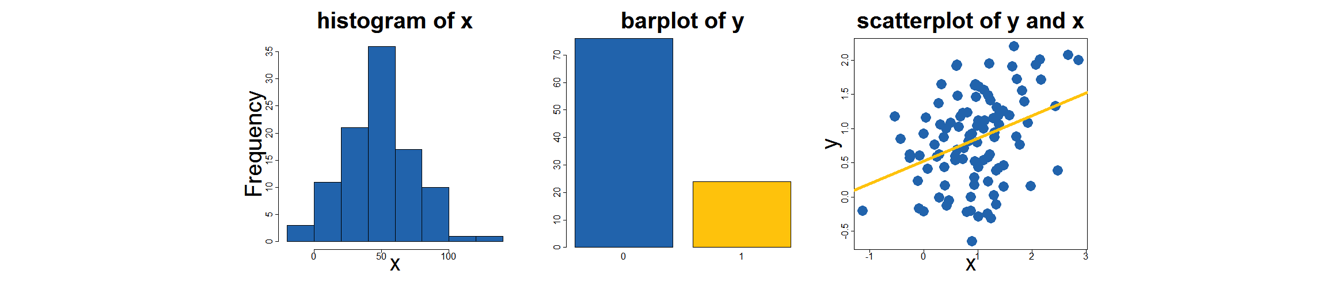
Figure 2.1: Graphical Possibilities in Base R
The
$sign is a kind of “connector”.mydata$xmeans: “The variablexin the dataset calledmydata”.
Sometimes, it is not necessary to use any options since some authors of R have done a good job of thinking about the defaults. R can make use of long pathnames to files like:
Note that R uses forward slashes
/instead of backslashes\for directories. R uses~to refer to the user’s (usually your) home directory.
3 Base R and Libraries
Most of this guide makes use of what is most often called Base R, the R that you get when you install the R software, and RStudio, on your computer.
For many social researchers, the data structure of primary interest is the data frame, and thus that is my focus here. In the interests of parsimony I do not go into a great deal of detail on R’s other data structures.
A great deal can be accomplished with Base R. However, as you grow in your use of R, you will likely frequently need to make use of libraries, which are invoked by the library(...) command.
Before using a library you need to install it. Below is an example of installing the ggplot2 advanced graphics library.
You would need to install the library only once. Installation can also be accomplished from the “Packages” tab in RStudio.
Then start the library when you are using R by typing…
I should mention here the new additions to the R language of the new libraries which make up the tidyverse. Learning the tidyverse requires an additional investment in learning, however the tidyverse makes many improvements to the R language and functionality.
4 Working Directory
R uses the concept of a working directory to know where to find files, and where to save files.
It is often helpful to simply set your working directory to a particular location and by default, files will be accessed from, and saved to, that directory e.g.:
getwd() # "get", or find out, your working directory

setwd("C:/Users/user1/Desktop/") # set your working directory
Note that R uses a forward slash
/to specify directory paths. R does not understand the use of a backward slash\to specify directories. R uses~to refer to the user’s (usually your) home directory.
5 Writing R Code or Script
R is a command or syntax based program, and many advanced functions are only available via syntax.
R Commands are stored in a script or code file that usually ends in .R, e.g.
myRscript.R. The command file is distinct from your actual data, stored in an .RData file, e.g.mydata.RData.
Base R can sometimes be cryptic.
However, a little bit of Base R can go a long way, and you can get a great learning return for a little bit of investment in learning Base R.
6 Graphical User Interface
A good Graphical User Interface (GUI) can make some of the base functionality of R available without the use of syntax. RCommander is the best GUI, and can be installed from the command line by typing:
RCommander can make some tasks easier, but the syntax that it produces can sometimes be non-intuitive. Often it is easiest (and more in the interests of replicable research) just to learn how to write the R code that accomplishes a particular task. Further, your learning may go quicker if you bypass RCommander altogether and simply learn how to write R code.
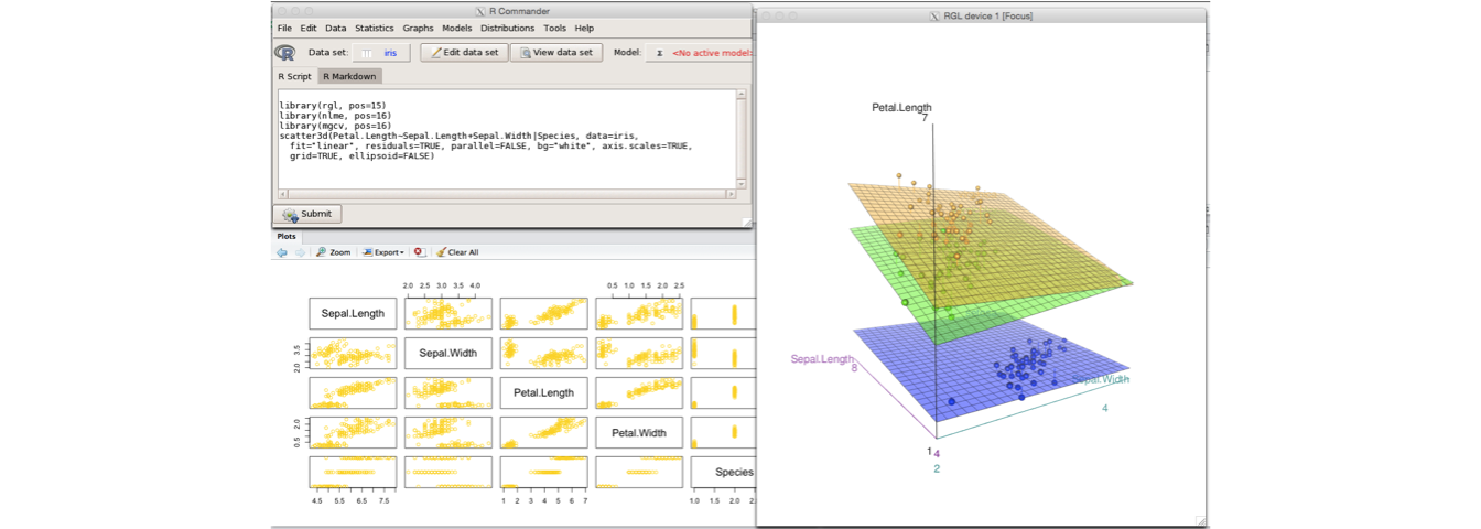
Figure 6.1: screenshot of RCommander
RStudio is an Integrated Development Environment (IDE) that can be run simultaneously with RCommander and provides an easier working enivronment for R Software. I
If all the software is installed, Start RStudio to start R, then type library(Rcmdr) to start RCommander.
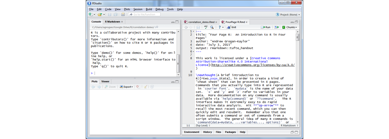
Figure 6.2: screenshot of RStudio
7 Get Your Data
Remember that R uses a forward slash
/to specify directory paths. R does not understand the use of a backward slash \(\backslash\) to specify directories.
7.1 R format (*.RData)
R most easily makes use of data in R format. Data can be loaded with the load() command.
load("the/path/to/myRfile.RData") # specific directory path and file

load("myRfile.RData") # no path indicated; file needs to be in working directory
Note–as we discuss in a little more detail below–that a single data file can contain multiple data frames.
For example, a data file called projectdata.RData could contain:
- A data frame on clients, called clients.
- A data frame on providers, called providers.
- A data frame on facilities, called facilities.
The name of the RData file can be very different from the name of the data frames that it contains.
7.3 Statistical Packages and Excel
R can easily import well-formatted data from other packages} like SPSS, Stata, or Excel2.
8 Save Your Data in R Format
Once you have your data in R, it will likely make sense to save it in *.RData format for future use.
Note–as we alluded to earlier–that multiple data frames can be saved into a single data file.3
9 Save and Document Your Work
Use the Script Editor to save R commands that you want to use again, or to modify for the next project, as well as to create an “audit trail” of your work so that your workflow is documented and replicable. R commands are saved in a .R file, e.g. myscript.R.
10 Process Your Data
10.1 Random Sample
Working with a random sample of your data can often be helpful.
The exact syntax of the R sample command is notably non-intuitive.
10.2 Data Subsets
Working with a subset of your data (i.e. fewer variables rather than many many variables) is often helpful. The subset function can be especially helpful.
mydata_subset <- subset(mydata, # name of data
                        age > 18, # condition(s)
                        select = c(id, sex, income)) # variables
You can then run functions like summary() on a subset of your data.
You can also save this subset for future use.
10.3 Numeric and Factor Variables
R recognizes two basic kinds of variables: continuous variables (which R calls numeric variables) which are often scales like income, mental health, or neighborhood quality; and categorical variables (which R calls factor variables) like race, gender or religion.
R seems to make a stronger distinction between these two types of variables than some other statistical software.4
Before changing your variables use summary to check their variable type.
x1 is numeric.
##    Min. 1st Qu.  Median    Mean 3rd Qu.    Max.
##   74.50   92.43   99.10   99.29  105.67  125.97
x2 is a factor.
##  0  1
## 74 26
It can sometimes be useful to change variables from one type to another.
If a factor variable has labels for the different levels, we can add those as well.
# longer, more complete syntax

mydata$w <- factor(mydata$z, # original numeric variable
                   levels = c(0, 1, 2), # levels of numeric variable
                   labels = c("Group A", # labels
                              "Group B",
                              "Group C"),
                   ordered = TRUE) # often useful to order the levels
Lastly, it may sometimes be helpful–especially for graphing–to reorder the levels of a factor.
Or, when the levels are in text:
10.4 Missing Values
Data with missing values, often represented as negative numbers (e.g. -99, -9, -8) need to be recoded so that the missing values are represented as a missing value character (“NA”) that R knows to exclude from calculations.
Sometimes you want to drop rows of data that contain missing values. This can be accomplished with na.omit().
na.omit() removes a row of data where any value is missing, so sometimes you want to work with a subset of your data before applying na.omit().
10.5 Renaming Variables
It is often convenient to rename your data so that the variables have more intuitively understandable names e.g.
10.6 Sorting Data
It is sometimes useful to sort your data. sort(mydata$x) will sort mydata by the values of x.
10.7 Creating New Variables
You can easily create new variables in R. For example, a change score between a measure collected at two time-points, like a pre-test, and a post-test, would be:
10.8 Recoding Variables
We can recode variables in R using R’s conditional syntax: dataset$variable[condition] <- value5 as in the example below.
Below we create a new variable ynew based upon the value of y.
11 Descriptive Statistics
11.1 Continuous Variables
summary(mydata$x) gives you basic descriptive statistics for a variable, such as the mean (average). Especially useful for continuous variables. Use summary(mydata) to summarize every variable in your data.
skim(mydata) from library(skimr) or describe(mydata) from library(psych) will often give you a nicer summary of your variables that is closer to what you want for an academic paper or agency report.
describe(mydata) is often especially useful when you want to show both the mean and standard deviation for several variables.
11.2 Categorical Variables
table(mydata$x) gives you a frequency distribution for your variable. Especially useful for factor variables.
prop.table(table(mydata$x)) will give you a table of proportions.
Calling up library(descr) and then using freq(mydata$x) will give you a more nicely formatted frequency distribution.
You may only want to look at descriptive statistics for a subset of your data. Creating a subset and then running descriptive statistics on that subset may be helpful.
11.3 Scientific Notation
R will, by default, often make use of scientific notation to express very large, or very small numbers, e.g. \(1.03 \times 10^7\) instead of \(1,030,000\), or \(1.03 \times 10^{-7}\) to express \(.000000103\).
Sometimes you will want to turn off this use of scientific notation.
12 Bivariate Statistics
12.1 Crosstabulation
Tabulating two categorical variables (factor variables) together gives you a cross-tabulation of those variables, e.g:
table(mydata$x, mydata$y) # simple table of counts

prop.table(table(mydata$x, mydata$y)) # table of cell proportions

prop.table(table(mydata$x, mydata$y),
           margin = 1) # row margins: row proportions

prop.table(table(mydata$x, mydata$y),
           margin = 2) # column margins: column proportions
then
will give you a chi-square test of the relationship of x and y.
12.2 Correlation
The easiest way to test a correlation in R seems to be to create a subset of the data that contains the variables for which you are interested in testing the correlation.
will test the statistical significance of this correlation.
14 Graphing
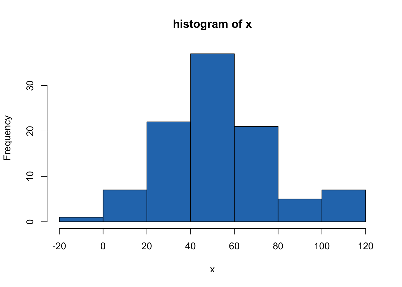
Figure 14.1: histogram of x
will give you a nice display of one continuous variable.
gives a nicer looking graph.
gives similar results when x is a factor variable.
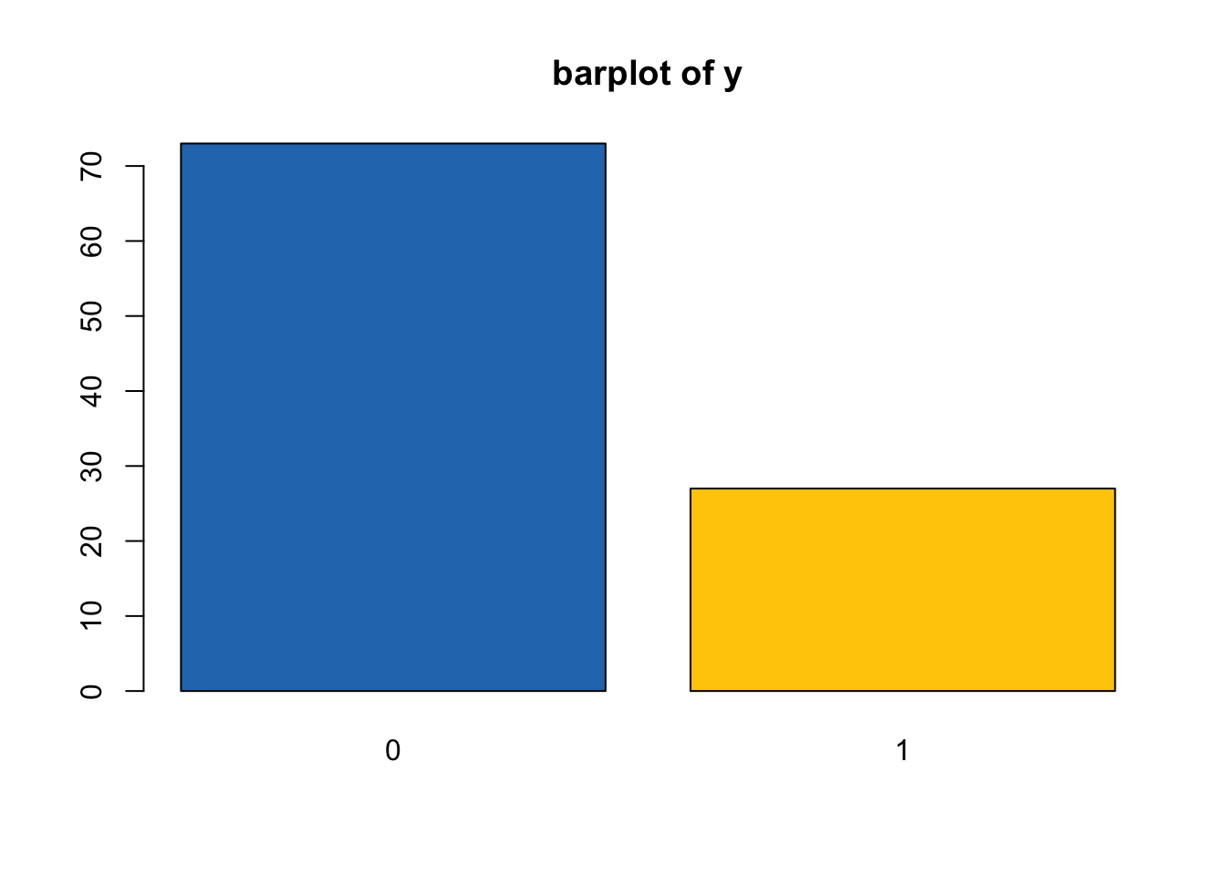
Figure 14.2: barplot of y
gives you a twoway scatterplot of your data
A more nicely labelled graph can be obtained with:
abline(lm(mydata$y~mydata$x)) will add a linear fit line to a scatterplot that you have already constructed.
abline(lm(mydata$y~mydata$x), col="gold", lwd=5) will be a nicer looking fit line.
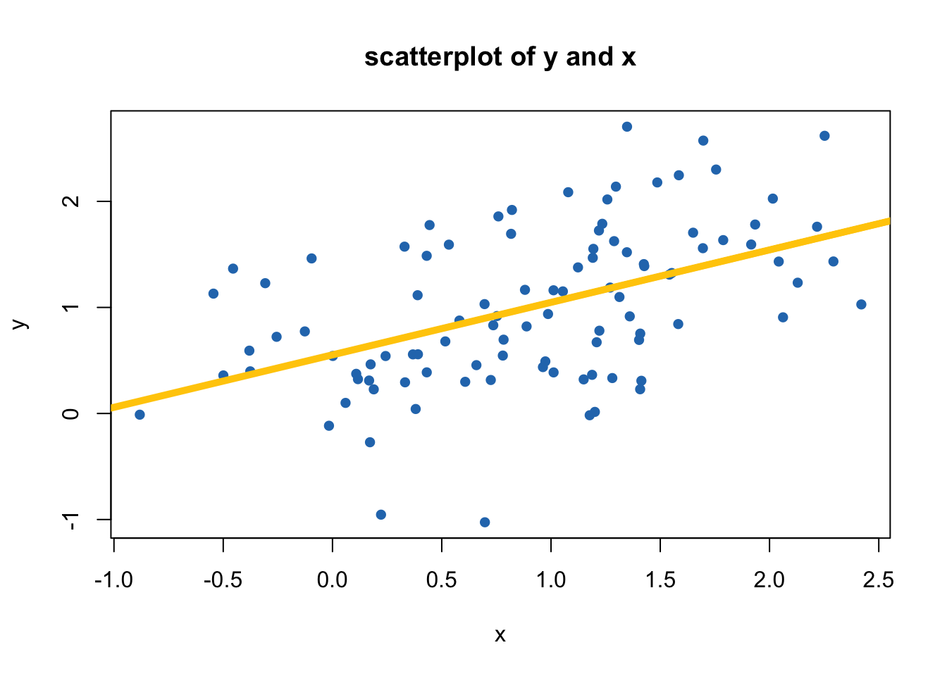
Figure 14.3: scatterplot of y against x
This document is inspired by my longstanding “Two Page Stata” document: (PDF) (HTML).↩︎
These instructions assume you have
setwd()appropriately, or alternatively are specifying a full pathname and filename.↩︎Some would call this a feature of R, while others would simply say that this is another confusing aspect of R.↩︎
In many cases, this is very helpful in that R recognizes that the type of variable calls for a certain kind of statistic or graph, or vice versa. In other cases, this may be the source of an error message.↩︎
Remember that while
>is used to test whetherx > y,<is used to test whetherx < y,==is required to test equality:x == y.↩︎
15 Comments, Questions and Corrections
Comments, questions and corrections most welcome and may be sent to: Andrew Grogan-Kaylor @ http://www.umich.edu/~agrogan & @ agrogan@umich.edu.
Last updated:
March 31 2026at15:19