dplyr is a very powerful R library for managing and processing data.1
While dplyr is very powerful, learning to use dplyr can be very confusing. This guide aims to present some of the most common dplyr functions and commands in the form of a brief cheatsheet.
library(dplyr) # data wrangling
2 Simulated Data
year
x
y
z
2019
NA
Group B
90
2020
50
Group C
90
2020
NA
Group A
100
2021
70
Group A
110
2021
80
Group B
120
3 Piping
Pipes%>% connect pieces of a command e.g. data to data wrangling to a graph command.
dplyr commands will often look something like the outline below.
newdata <- mydata %>%filter(!is.na(x)) # filter by x is not missing
year
x
y
z
2020
50
Group C
90
2021
70
Group A
110
2021
80
Group B
120
11 Random Sample
newdata <- mydata %>%sample_frac(.5) # fraction of data to sample
year
x
y
z
2021
70
Group A
110
2020
50
Group C
90
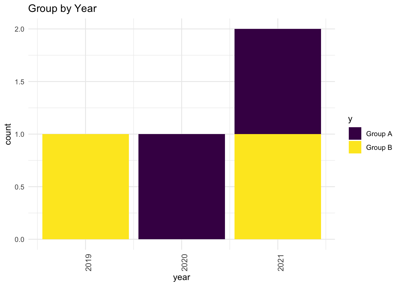
12 Connecting To Other Packages Like ggplot
Notice how, in the code below, I never actually create the new data set mynewdata. I simply pipe mydata into a dplyr command, and pipe the result directly to ggplot2.
library(ggplot2)mydata %>%# my datamutate(myscale = x + z) %>%# dplyr command to make new variable filter(y !="Group C") %>%# filter on values of yggplot(aes(x = year, # the rest is ggplotfill = y)) +geom_bar() +scale_fill_viridis_d(option ="viridis") +# viridis colorstheme_minimal() +# minimal themelabs(title ="Group by Year") +# labelstheme(axis.text.x =element_text(size =10, # tweak themeangle =90))
Footnotes
The origins of the name dplyr seem somewhat obscure, but I sometimes think of this package as the data plyers.↩︎