Introduction

• Stata is a powerful and intuitive data analysis program.
• Learning how to graph in Stata is an important part of learning how to use Stata.
• Yet, the default graphs in Stata can sometimes be less than optimal.
• This document is an introduction to (a) basic graphing ideas in Stata; and (b) some simple ways to make your Stata graphs look more professional.

What are Variables?

• By variables, I simply mean the columns of data that you have.
• For our purposes, you may think of variables as synonymous with questionnaire items, or columns of data.

Variable Types

• categorical variables represent unordered categories like neighborhood, or religious affiliation, or place of residence.
• continuous variables represent a continuous scale like a mental health scale, or a measure of life expectancy.

A Data Visualization Strategy

Once we have discerned the type of variable that have, there are two followup questions we may ask before deciding upon a chart strategy:

• Is our graph about one thing at a time?
  • How much of x is there?
  • What is the distribution of x?
• Is our graph about two things at a time?
  • What is the relationship of x and y?
  • How are x and y associated?

Data

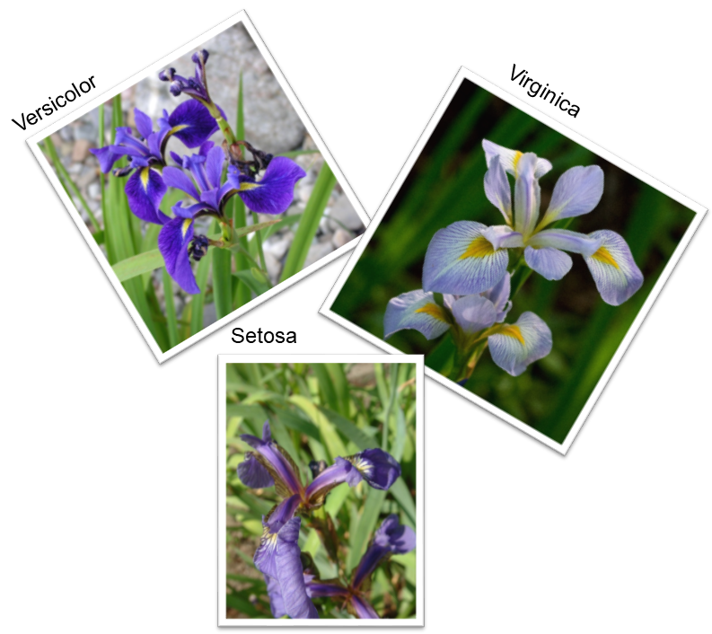
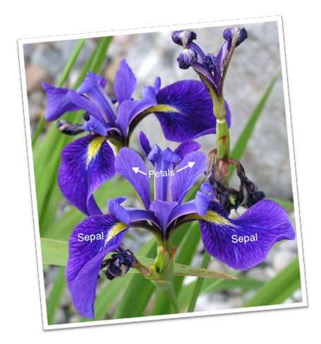
We are going to use the famous “iris” data collected by Edgar Anderson in the early 20th Century.

. use "iris.dta", clear

. 
. summarize

    Variable │        Obs        Mean    Std. dev.       Min        Max
─────────────┼─────────────────────────────────────────────────────────
Sepal_Length │        150    5.843333    .8280661        4.3        7.9
 Sepal_Width │        150    3.057333    .4358663          2        4.4
Petal_Length │        150       3.758    1.765298          1        6.9
 Petal_Width │        150    1.199333    .7622377         .1        2.5
     Species │        150           2    .8192319          1          3

The iris data set has 5 variables.

Species of Iris

Iris species images courtesy Wikipedia.

Petals and Sepals

Basic Graphs

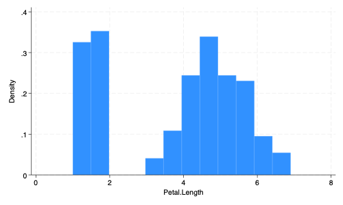
Continuous Variable histogram

. histogram Petal_Length
(bin=12, start=1, width=.49166667)

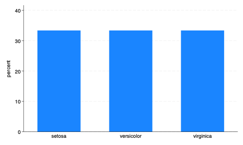
Categorical Variable graph bar

. graph bar, over(Species)

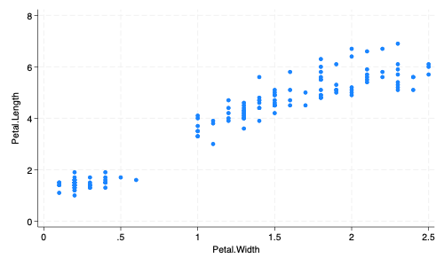
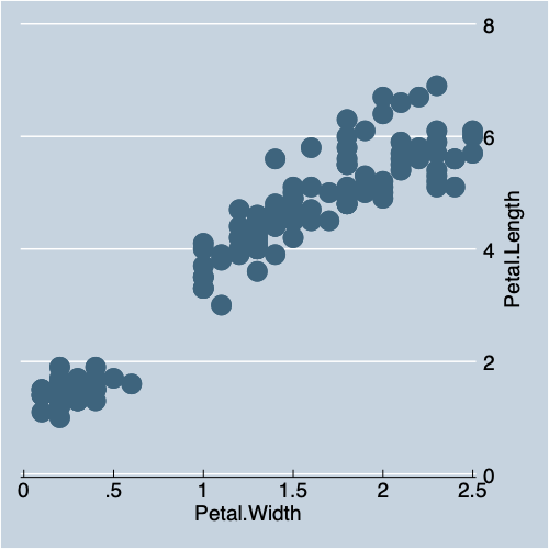
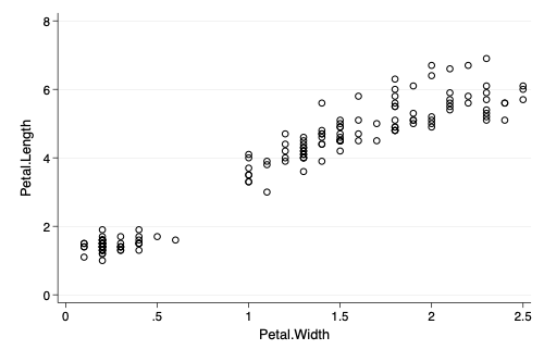
Continuous by Continuous twoway

. twoway scatter Petal_Length Petal_Width

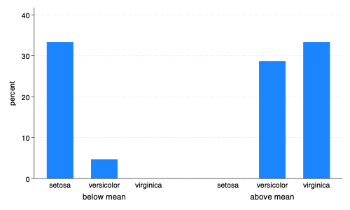
Categorical by Categorical graph bar

. recode Petal_Length ///
> (min/3.758 = 0 "below mean") ///
> (3.758/max = 1 "above mean"), ///
> generate(Petal_Group) // dichotomize Petal_Length
(150 differences between Petal_Length and Petal_Group)

.     
. graph bar, over(Species) over(Petal_Group)

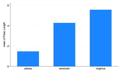
Continuous by Categorical graph bar

. graph bar Petal_Length, over(Species)

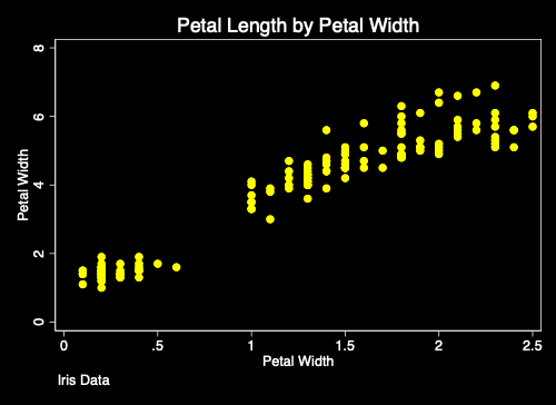
Titles and Labels , title(...) xtitle(...) ytitle(...)

. twoway scatter Petal_Length Petal_Width, scheme(s1rcolor) ///
> title("Petal Length by Petal Width") ///
> xtitle("Petal Width") ytitle("Petal Width") ///
> caption("Iris Data") 

Better Graphing With Schemes ,scheme(...)

The easiest method to make better Stata graphs is through the use of predefined Stata graphing schemes.

Pre-Defined Schemes

Some schemes, e.g. economist, sj, s1color, and s1rcolor are pre-installed with Stata.

Economist Scheme

. twoway scatter Petal_Length Petal_Width, scheme(economist)

Stata Journal Scheme

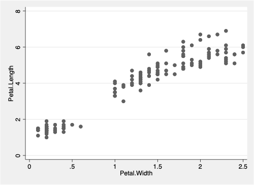
. twoway scatter Petal_Length Petal_Width, scheme(sj)

s1color Scheme

. twoway scatter Petal_Length Petal_Width, scheme(s1color)

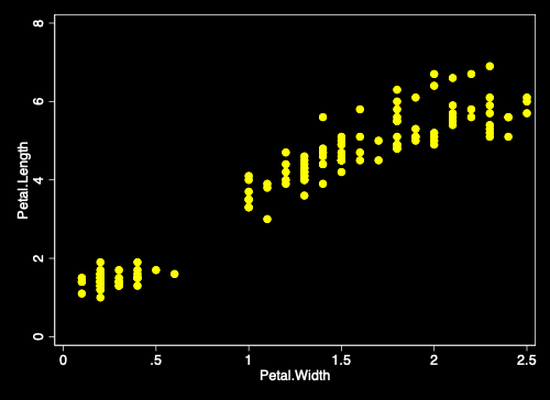
s1rcolor Scheme

. twoway scatter Petal_Length Petal_Width, scheme(s1rcolor)

User Written Schemes

Two of the best user written schemes are plottig and lean2.

Use the findit command e.g. findit lean2 to find these schemes.

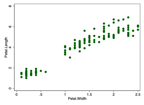
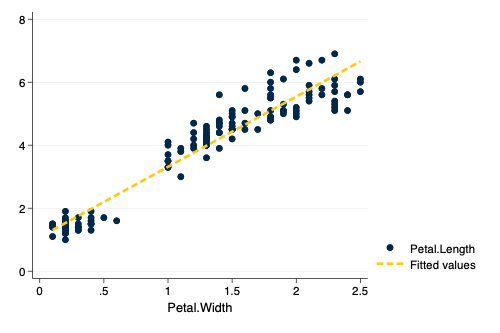
lean2 Scheme

. twoway scatter Petal_Length Petal_Width, scheme(lean2)

Michigan graph scheme

I have written a michigan graph scheme described here.

. twoway (scatter Petal_Length Petal_Width) /// 
> (lfit Petal_Length Petal_Width), scheme(michigan)

Schemes as a Base for Further Tweaking

Schemes can be used as a base that can then be further modified.

. twoway (scatter Petal_Length Petal_Width, msymbol(0) mcolor(red)) ///
> (lfit Petal_Length Petal_Width), ///
> scheme(lean2) 
(note:  named style 0 not found in class symbol, default attributes used)

Even More Tweaks

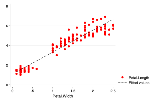
Based upon an example at https://blog.stata.com/2018/10/02/scheming-your-way-to-your-favorite-graph-style/

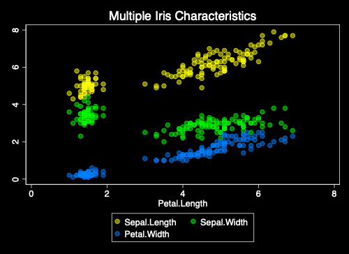
. twoway scatter Sepal_Length Sepal_Width Petal_Width Petal_Length, /// 
> color(%50 %50 %50) /// transparency 
> title("Multiple Iris Characteristics") /// title
> scheme(s1rcolor) // scheme

More Information

See also Two Page Stata

Created by agrogan@umich.edu