Set Up 🌲

You will need to install the relevant packages: lme4 for frequentist MLM, and brms, which also installs STAN, for Bayesian MLM.

Show code

install.packages(c("lme4", "brms"))

Gutten Tree Data 🌲

Norway Spruce and Larch Forest in Austrian Alps, https://ec.europa.eu/jrc/en/research-topic/forestry/qr-tree-project/norway-spruce

The data used in this example are derived from the R package Functions and Datasets for “Forest Analytics with R”.

According to the documentation, the source of these data are: “von Guttenberg’s Norway spruce (Picea abies [L.] Karst) tree measurement data.”

The documentation goes on to further note that:

“The data are measures from 107 trees. The trees were selected as being of average size from healthy and well stocked stands in the Alps.”

Import The Data 🌲

Show code

library(haven)

gutten <- read_dta("gutten.dta")

gutten

# A tibble: 1,200 × 9
      site location  tree age_base height dbh_cm volume age_bh tree_ID
   <dbl+l> <dbl+lb> <dbl>    <dbl>  <dbl>  <dbl>  <dbl>  <dbl> <dbl+l>
 1   1 [1]    1 [1]     1       20    4.2    4.6      5   9.67 1 [1.1]
 2   1 [1]    1 [1]     1       30    9.3   10.2     38  19.7  1 [1.1]
 3   1 [1]    1 [1]     1       40   14.9   14.9    123  29.7  1 [1.1]
 4   1 [1]    1 [1]     1       50   19.7   18.3    263  39.7  1 [1.1]
 5   1 [1]    1 [1]     1       60   23     20.7    400  49.7  1 [1.1]
 6   1 [1]    1 [1]     1       70   25.8   22.6    555  59.7  1 [1.1]
 7   1 [1]    1 [1]     1       80   27.4   24.1    688  69.7  1 [1.1]
 8   1 [1]    1 [1]     1       90   28.8   25.5    820  79.7  1 [1.1]
 9   1 [1]    1 [1]     1      100   30     26.5    928  89.7  1 [1.1]
10   1 [1]    1 [1]     1      110   30.9   27.3   1023  99.7  1 [1.1]
# … with 1,190 more rows

Variables 🌲

site Growth quality class of the tree’s habitat. 5 levels.

location Distinguishes tree location. 7 levels.

tree An identifier for the tree within location.

age.base The tree age taken at ground level.

height Tree height, m.

dbh.cm Tree diameter, cm.

volume Tree volume.

age.bh Tree age taken at 1.3 m.

tree.ID A factor uniquely identifying the tree.

A Basic Multilevel Model 🌲

\[\text{height}_{it} = \beta_0 + \beta \text{age_base} + \beta \text{site} + \beta \text{age_base * site} + u_{0\text{ tree.ID}} + e_{it}\] Both lmer (frequentist MLM) and brms (Bayesian MLM) use the idea of translating the above equation into a formula:

height ~ age_base + site + (1 | tree_ID)

Graph (Spaghetti Plot)

Show code

library(ggplot2)

ggplot(gutten,
       aes(x = age_base, # x is tree age
           y = height)) + # y is tree height
  geom_smooth(aes(color = as.factor(tree_ID)), 
              method = "lm",
              se = FALSE) + # linear model for each tree
  geom_smooth(method = "lm", 
              color = "red",
              size = 2) + # linear model 
  labs(title = "Tree Height As A Function Of Age") +
  scale_color_viridis_d() + # nice graph colors for trees
  theme_minimal() +
  theme(legend.position = "none")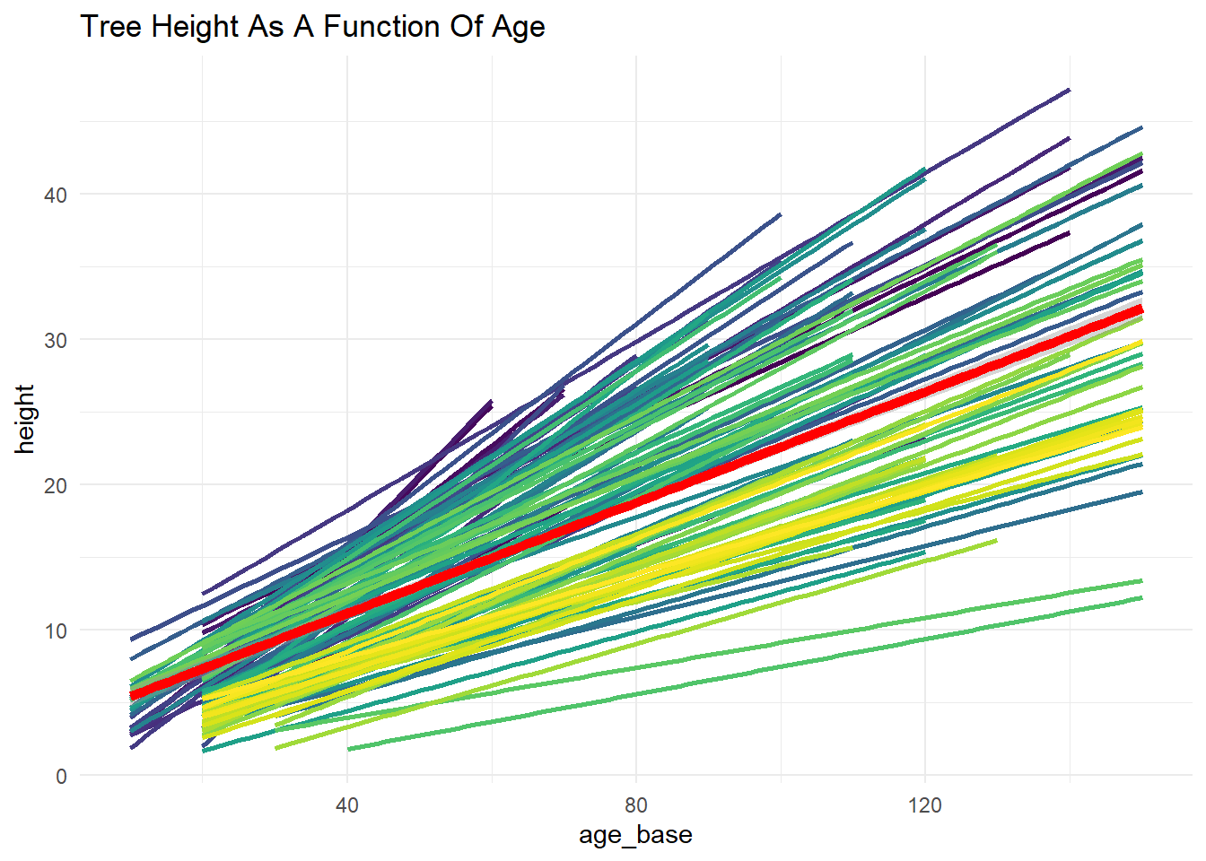

Frequentist Model in `lmer` 🌲

NB: * provides with an interaction term and main effects.

Show code

library(lme4)

fit1 <- lmer(height ~ age_base * site + (1 | tree_ID), 
             data = gutten)

summary(fit1)

Linear mixed model fit by REML ['lmerMod']
Formula: height ~ age_base * site + (1 | tree_ID)
   Data: gutten

REML criterion at convergence: 5565.2

Scaled residuals: 
    Min      1Q  Median      3Q     Max 
-3.7145 -0.5346  0.1588  0.6739  2.5713 

Random effects:
 Groups   Name        Variance Std.Dev.
 tree_ID  (Intercept) 2.462    1.569   
 Residual             5.037    2.244   
Number of obs: 1200, groups:  tree_ID, 107

Fixed effects:
               Estimate Std. Error t value
(Intercept)    4.736446   0.497759   9.516
age_base       0.324732   0.004449  72.990
site          -1.013740   0.175037  -5.792
age_base:site -0.040400   0.001488 -27.154

Correlation of Fixed Effects:
            (Intr) age_bs site  
age_base    -0.610              
site        -0.906  0.546       
age_base:st  0.574 -0.910 -0.625

Bayesian Model With `brms` (Less Informative Default Priors) 🌲

The models below take a non-trivial amount of time to run.

Show code

library(brms)

fit2 <- brm(height ~ age_base * site + (1 | tree_ID), 
            data = gutten,
            family = gaussian(), 
            warmup = 2000, 
            iter = 5000)


SAMPLING FOR MODEL '7b48f719fba0583cf851dcec2120d203' NOW (CHAIN 1).
Chain 1: 
Chain 1: Gradient evaluation took 0.000288 seconds
Chain 1: 1000 transitions using 10 leapfrog steps per transition would take 2.88 seconds.
Chain 1: Adjust your expectations accordingly!
Chain 1: 
Chain 1: 
Chain 1: Iteration:    1 / 5000 [  0%]  (Warmup)
Chain 1: Iteration:  500 / 5000 [ 10%]  (Warmup)
Chain 1: Iteration: 1000 / 5000 [ 20%]  (Warmup)
Chain 1: Iteration: 1500 / 5000 [ 30%]  (Warmup)
Chain 1: Iteration: 2000 / 5000 [ 40%]  (Warmup)
Chain 1: Iteration: 2001 / 5000 [ 40%]  (Sampling)
Chain 1: Iteration: 2500 / 5000 [ 50%]  (Sampling)
Chain 1: Iteration: 3000 / 5000 [ 60%]  (Sampling)
Chain 1: Iteration: 3500 / 5000 [ 70%]  (Sampling)
Chain 1: Iteration: 4000 / 5000 [ 80%]  (Sampling)
Chain 1: Iteration: 4500 / 5000 [ 90%]  (Sampling)
Chain 1: Iteration: 5000 / 5000 [100%]  (Sampling)
Chain 1: 
Chain 1:  Elapsed Time: 9.74825 seconds (Warm-up)
Chain 1:                5.9866 seconds (Sampling)
Chain 1:                15.7349 seconds (Total)
Chain 1: 

SAMPLING FOR MODEL '7b48f719fba0583cf851dcec2120d203' NOW (CHAIN 2).
Chain 2: 
Chain 2: Gradient evaluation took 6.7e-05 seconds
Chain 2: 1000 transitions using 10 leapfrog steps per transition would take 0.67 seconds.
Chain 2: Adjust your expectations accordingly!
Chain 2: 
Chain 2: 
Chain 2: Iteration:    1 / 5000 [  0%]  (Warmup)
Chain 2: Iteration:  500 / 5000 [ 10%]  (Warmup)
Chain 2: Iteration: 1000 / 5000 [ 20%]  (Warmup)
Chain 2: Iteration: 1500 / 5000 [ 30%]  (Warmup)
Chain 2: Iteration: 2000 / 5000 [ 40%]  (Warmup)
Chain 2: Iteration: 2001 / 5000 [ 40%]  (Sampling)
Chain 2: Iteration: 2500 / 5000 [ 50%]  (Sampling)
Chain 2: Iteration: 3000 / 5000 [ 60%]  (Sampling)
Chain 2: Iteration: 3500 / 5000 [ 70%]  (Sampling)
Chain 2: Iteration: 4000 / 5000 [ 80%]  (Sampling)
Chain 2: Iteration: 4500 / 5000 [ 90%]  (Sampling)
Chain 2: Iteration: 5000 / 5000 [100%]  (Sampling)
Chain 2: 
Chain 2:  Elapsed Time: 11.4588 seconds (Warm-up)
Chain 2:                6.64869 seconds (Sampling)
Chain 2:                18.1075 seconds (Total)
Chain 2: 

SAMPLING FOR MODEL '7b48f719fba0583cf851dcec2120d203' NOW (CHAIN 3).
Chain 3: 
Chain 3: Gradient evaluation took 8.5e-05 seconds
Chain 3: 1000 transitions using 10 leapfrog steps per transition would take 0.85 seconds.
Chain 3: Adjust your expectations accordingly!
Chain 3: 
Chain 3: 
Chain 3: Iteration:    1 / 5000 [  0%]  (Warmup)
Chain 3: Iteration:  500 / 5000 [ 10%]  (Warmup)
Chain 3: Iteration: 1000 / 5000 [ 20%]  (Warmup)
Chain 3: Iteration: 1500 / 5000 [ 30%]  (Warmup)
Chain 3: Iteration: 2000 / 5000 [ 40%]  (Warmup)
Chain 3: Iteration: 2001 / 5000 [ 40%]  (Sampling)
Chain 3: Iteration: 2500 / 5000 [ 50%]  (Sampling)
Chain 3: Iteration: 3000 / 5000 [ 60%]  (Sampling)
Chain 3: Iteration: 3500 / 5000 [ 70%]  (Sampling)
Chain 3: Iteration: 4000 / 5000 [ 80%]  (Sampling)
Chain 3: Iteration: 4500 / 5000 [ 90%]  (Sampling)
Chain 3: Iteration: 5000 / 5000 [100%]  (Sampling)
Chain 3: 
Chain 3:  Elapsed Time: 14.3936 seconds (Warm-up)
Chain 3:                7.67574 seconds (Sampling)
Chain 3:                22.0693 seconds (Total)
Chain 3: 

SAMPLING FOR MODEL '7b48f719fba0583cf851dcec2120d203' NOW (CHAIN 4).
Chain 4: 
Chain 4: Gradient evaluation took 0.000142 seconds
Chain 4: 1000 transitions using 10 leapfrog steps per transition would take 1.42 seconds.
Chain 4: Adjust your expectations accordingly!
Chain 4: 
Chain 4: 
Chain 4: Iteration:    1 / 5000 [  0%]  (Warmup)
Chain 4: Iteration:  500 / 5000 [ 10%]  (Warmup)
Chain 4: Iteration: 1000 / 5000 [ 20%]  (Warmup)
Chain 4: Iteration: 1500 / 5000 [ 30%]  (Warmup)
Chain 4: Iteration: 2000 / 5000 [ 40%]  (Warmup)
Chain 4: Iteration: 2001 / 5000 [ 40%]  (Sampling)
Chain 4: Iteration: 2500 / 5000 [ 50%]  (Sampling)
Chain 4: Iteration: 3000 / 5000 [ 60%]  (Sampling)
Chain 4: Iteration: 3500 / 5000 [ 70%]  (Sampling)
Chain 4: Iteration: 4000 / 5000 [ 80%]  (Sampling)
Chain 4: Iteration: 4500 / 5000 [ 90%]  (Sampling)
Chain 4: Iteration: 5000 / 5000 [100%]  (Sampling)
Chain 4: 
Chain 4:  Elapsed Time: 11.2545 seconds (Warm-up)
Chain 4:                7.10916 seconds (Sampling)
Chain 4:                18.3637 seconds (Total)
Chain 4:

Show code

summary(fit2)

 Family: gaussian 
  Links: mu = identity; sigma = identity 
Formula: height ~ age_base * site + (1 | tree_ID) 
   Data: gutten (Number of observations: 1200) 
  Draws: 4 chains, each with iter = 5000; warmup = 2000; thin = 1;
         total post-warmup draws = 12000

Group-Level Effects: 
~tree_ID (Number of levels: 107) 
              Estimate Est.Error l-95% CI u-95% CI Rhat Bulk_ESS
sd(Intercept)     1.59      0.13     1.35     1.85 1.00     4012
              Tail_ESS
sd(Intercept)     6890

Population-Level Effects: 
              Estimate Est.Error l-95% CI u-95% CI Rhat Bulk_ESS
Intercept         4.74      0.50     3.77     5.73 1.00     4695
age_base          0.32      0.00     0.32     0.33 1.00    17134
site             -1.01      0.18    -1.36    -0.67 1.00     4710
age_base:site    -0.04      0.00    -0.04    -0.04 1.00    17388
              Tail_ESS
Intercept         7001
age_base          9915
site              5964
age_base:site     9255

Family Specific Parameters: 
      Estimate Est.Error l-95% CI u-95% CI Rhat Bulk_ESS Tail_ESS
sigma     2.25      0.05     2.15     2.34 1.00    21717     9392

Draws were sampled using sampling(NUTS). For each parameter, Bulk_ESS
and Tail_ESS are effective sample size measures, and Rhat is the potential
scale reduction factor on split chains (at convergence, Rhat = 1).

Set Informative Priors 🌲

Show code

prior1 <- c(
  prior(normal(0, 10), class = Intercept), 
  prior(normal(0, 10), class = b, coef = site) #,
  # prior(cauchy(0, 10), class = sigma)
)

Run The Model With More Informative Prior 🌲

Show code

fit3 <- brm(height ~ age_base * site + (1 | tree_ID), 
            data = gutten,
            family = gaussian(), 
            prior = prior1,
            warmup = 2000, 
            iter = 5000)


SAMPLING FOR MODEL 'afee0b50f733aec486aeaaee2414cd7a' NOW (CHAIN 1).
Chain 1: 
Chain 1: Gradient evaluation took 0.000323 seconds
Chain 1: 1000 transitions using 10 leapfrog steps per transition would take 3.23 seconds.
Chain 1: Adjust your expectations accordingly!
Chain 1: 
Chain 1: 
Chain 1: Iteration:    1 / 5000 [  0%]  (Warmup)
Chain 1: Iteration:  500 / 5000 [ 10%]  (Warmup)
Chain 1: Iteration: 1000 / 5000 [ 20%]  (Warmup)
Chain 1: Iteration: 1500 / 5000 [ 30%]  (Warmup)
Chain 1: Iteration: 2000 / 5000 [ 40%]  (Warmup)
Chain 1: Iteration: 2001 / 5000 [ 40%]  (Sampling)
Chain 1: Iteration: 2500 / 5000 [ 50%]  (Sampling)
Chain 1: Iteration: 3000 / 5000 [ 60%]  (Sampling)
Chain 1: Iteration: 3500 / 5000 [ 70%]  (Sampling)
Chain 1: Iteration: 4000 / 5000 [ 80%]  (Sampling)
Chain 1: Iteration: 4500 / 5000 [ 90%]  (Sampling)
Chain 1: Iteration: 5000 / 5000 [100%]  (Sampling)
Chain 1: 
Chain 1:  Elapsed Time: 11.4875 seconds (Warm-up)
Chain 1:                6.9533 seconds (Sampling)
Chain 1:                18.4408 seconds (Total)
Chain 1: 

SAMPLING FOR MODEL 'afee0b50f733aec486aeaaee2414cd7a' NOW (CHAIN 2).
Chain 2: 
Chain 2: Gradient evaluation took 6.8e-05 seconds
Chain 2: 1000 transitions using 10 leapfrog steps per transition would take 0.68 seconds.
Chain 2: Adjust your expectations accordingly!
Chain 2: 
Chain 2: 
Chain 2: Iteration:    1 / 5000 [  0%]  (Warmup)
Chain 2: Iteration:  500 / 5000 [ 10%]  (Warmup)
Chain 2: Iteration: 1000 / 5000 [ 20%]  (Warmup)
Chain 2: Iteration: 1500 / 5000 [ 30%]  (Warmup)
Chain 2: Iteration: 2000 / 5000 [ 40%]  (Warmup)
Chain 2: Iteration: 2001 / 5000 [ 40%]  (Sampling)
Chain 2: Iteration: 2500 / 5000 [ 50%]  (Sampling)
Chain 2: Iteration: 3000 / 5000 [ 60%]  (Sampling)
Chain 2: Iteration: 3500 / 5000 [ 70%]  (Sampling)
Chain 2: Iteration: 4000 / 5000 [ 80%]  (Sampling)
Chain 2: Iteration: 4500 / 5000 [ 90%]  (Sampling)
Chain 2: Iteration: 5000 / 5000 [100%]  (Sampling)
Chain 2: 
Chain 2:  Elapsed Time: 10.1329 seconds (Warm-up)
Chain 2:                7.19358 seconds (Sampling)
Chain 2:                17.3265 seconds (Total)
Chain 2: 

SAMPLING FOR MODEL 'afee0b50f733aec486aeaaee2414cd7a' NOW (CHAIN 3).
Chain 3: 
Chain 3: Gradient evaluation took 0.000101 seconds
Chain 3: 1000 transitions using 10 leapfrog steps per transition would take 1.01 seconds.
Chain 3: Adjust your expectations accordingly!
Chain 3: 
Chain 3: 
Chain 3: Iteration:    1 / 5000 [  0%]  (Warmup)
Chain 3: Iteration:  500 / 5000 [ 10%]  (Warmup)
Chain 3: Iteration: 1000 / 5000 [ 20%]  (Warmup)
Chain 3: Iteration: 1500 / 5000 [ 30%]  (Warmup)
Chain 3: Iteration: 2000 / 5000 [ 40%]  (Warmup)
Chain 3: Iteration: 2001 / 5000 [ 40%]  (Sampling)
Chain 3: Iteration: 2500 / 5000 [ 50%]  (Sampling)
Chain 3: Iteration: 3000 / 5000 [ 60%]  (Sampling)
Chain 3: Iteration: 3500 / 5000 [ 70%]  (Sampling)
Chain 3: Iteration: 4000 / 5000 [ 80%]  (Sampling)
Chain 3: Iteration: 4500 / 5000 [ 90%]  (Sampling)
Chain 3: Iteration: 5000 / 5000 [100%]  (Sampling)
Chain 3: 
Chain 3:  Elapsed Time: 9.21782 seconds (Warm-up)
Chain 3:                6.54974 seconds (Sampling)
Chain 3:                15.7676 seconds (Total)
Chain 3: 

SAMPLING FOR MODEL 'afee0b50f733aec486aeaaee2414cd7a' NOW (CHAIN 4).
Chain 4: 
Chain 4: Gradient evaluation took 7.3e-05 seconds
Chain 4: 1000 transitions using 10 leapfrog steps per transition would take 0.73 seconds.
Chain 4: Adjust your expectations accordingly!
Chain 4: 
Chain 4: 
Chain 4: Iteration:    1 / 5000 [  0%]  (Warmup)
Chain 4: Iteration:  500 / 5000 [ 10%]  (Warmup)
Chain 4: Iteration: 1000 / 5000 [ 20%]  (Warmup)
Chain 4: Iteration: 1500 / 5000 [ 30%]  (Warmup)
Chain 4: Iteration: 2000 / 5000 [ 40%]  (Warmup)
Chain 4: Iteration: 2001 / 5000 [ 40%]  (Sampling)
Chain 4: Iteration: 2500 / 5000 [ 50%]  (Sampling)
Chain 4: Iteration: 3000 / 5000 [ 60%]  (Sampling)
Chain 4: Iteration: 3500 / 5000 [ 70%]  (Sampling)
Chain 4: Iteration: 4000 / 5000 [ 80%]  (Sampling)
Chain 4: Iteration: 4500 / 5000 [ 90%]  (Sampling)
Chain 4: Iteration: 5000 / 5000 [100%]  (Sampling)
Chain 4: 
Chain 4:  Elapsed Time: 11.6999 seconds (Warm-up)
Chain 4:                6.1912 seconds (Sampling)
Chain 4:                17.8911 seconds (Total)
Chain 4:

Show code

summary(fit3)

 Family: gaussian 
  Links: mu = identity; sigma = identity 
Formula: height ~ age_base * site + (1 | tree_ID) 
   Data: gutten (Number of observations: 1200) 
  Draws: 4 chains, each with iter = 5000; warmup = 2000; thin = 1;
         total post-warmup draws = 12000

Group-Level Effects: 
~tree_ID (Number of levels: 107) 
              Estimate Est.Error l-95% CI u-95% CI Rhat Bulk_ESS
sd(Intercept)     1.59      0.13     1.35     1.87 1.00     3989
              Tail_ESS
sd(Intercept)     7092

Population-Level Effects: 
              Estimate Est.Error l-95% CI u-95% CI Rhat Bulk_ESS
Intercept         4.72      0.50     3.73     5.70 1.00     4864
age_base          0.32      0.00     0.32     0.33 1.00    15193
site             -1.01      0.18    -1.36    -0.66 1.00     4679
age_base:site    -0.04      0.00    -0.04    -0.04 1.00    15305
              Tail_ESS
Intercept         7287
age_base          9877
site              6572
age_base:site     9415

Family Specific Parameters: 
      Estimate Est.Error l-95% CI u-95% CI Rhat Bulk_ESS Tail_ESS
sigma     2.25      0.05     2.15     2.34 1.00    20932     8889

Draws were sampled using sampling(NUTS). For each parameter, Bulk_ESS
and Tail_ESS are effective sample size measures, and Rhat is the potential
scale reduction factor on split chains (at convergence, Rhat = 1).

Plot Posterior Distributions and Trace Plots 🌲

plot(fit3) will give me a reasonable plot of every parameter, but the layout may not be optimal. I am using separate plot calls below, but to do so, I need to know the names of the parameters, which can be tricky in brms. One way to do this is to use plot(fit3) to see all the parameter names, and then divide the single plot call into multiple plot calls to improve the layout.

Show code

# plot(fit3)

plot(fit3, variable = c("b_Intercept"))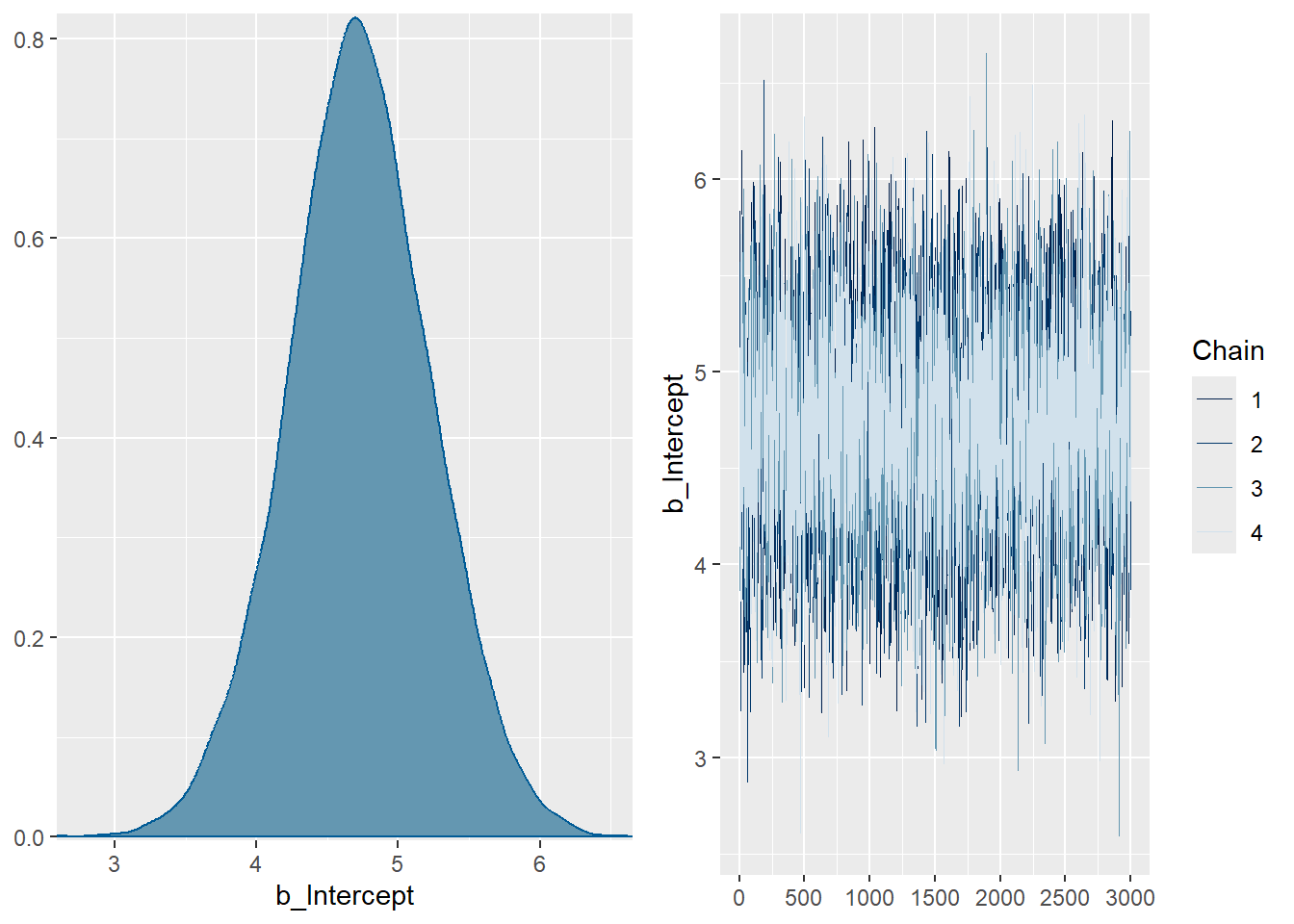

Show code

plot(fit3, 
     variable = c("b_age_base", 
                  "b_site",
                  "b_age_base:site")) # regression slopes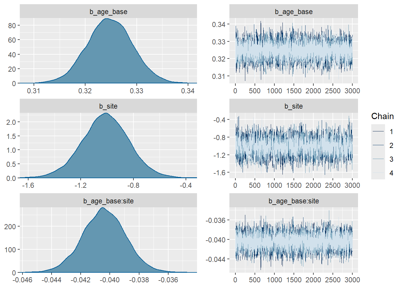

Show code

plot(fit3, variable = c("sd_tree_ID__Intercept",
                        "sigma")) # variance parameters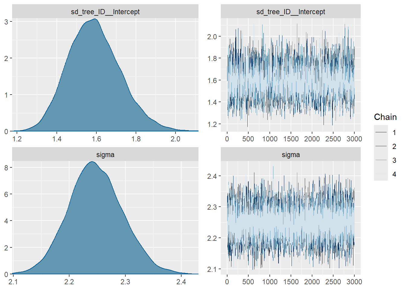

Compare All 3 Models 🌲

Show code

tab_model(fit1, fit2, fit3,
          dv.labels = c("lmer", "brms default priors", "brms informative priors"), 
          show.se = TRUE,
          show.ci = 0.95,
          show.stat = TRUE)

	lmer					brms default priors			brms informative priors
Predictors	Estimates	std. Error	CI	Statistic	p	Estimates	std. Error	CI (95%)	Estimates	std. Error	CI (95%)
(Intercept)	4.74	0.50	3.76 – 5.71	9.52	<0.001
age.base	0.32	0.00	0.32 – 0.33	72.99	<0.001	0.32	0.00	0.32 – 0.33	0.32	0.00	0.32 – 0.33
site	-1.01	0.18	-1.36 – -0.67	-5.79	<0.001	-1.01	0.17	-1.36 – -0.67	-1.01	0.18	-1.36 – -0.66
age_base:site	-0.04	0.00	-0.04 – -0.04	-27.15	<0.001	-0.04	0.00	-0.04 – -0.04	-0.04	0.00	-0.04 – -0.04
Intercept						4.73	0.49	3.77 – 5.73	4.73	0.51	3.73 – 5.70
Random Effects
σ²	5.04					5.05			5.05
τ₀₀	2.46 _{tree_ID}					2.51 _{tree_ID}			2.54 _{tree_ID}
ICC	0.33					0.33			0.33
N	107 _{tree_ID}					107 _{tree_ID}			107 _{tree_ID}
Observations	1200					1200			1200
Marginal R² / Conditional R²	0.916 / 0.944					0.915 / 0.941			0.915 / 0.941

Bayesian Longitudinal Multilevel Models

Set Up 🌲

Gutten Tree Data 🌲

Import The Data 🌲

Variables 🌲

A Basic Multilevel Model 🌲

Graph (Spaghetti Plot)

Frequentist Model in lmer 🌲

Bayesian Model With brms (Less Informative Default Priors) 🌲

Set Informative Priors 🌲

Run The Model With More Informative Prior 🌲

Plot Posterior Distributions and Trace Plots 🌲

Compare All 3 Models 🌲

Frequentist Model in `lmer` 🌲

Bayesian Model With `brms` (Less Informative Default Priors) 🌲