These notes represent a brief discussion of centering with cross
sectional data. Since so much of my current work focuses on cross
national work on parenting and child development, I use these ideas as
my substantive example.
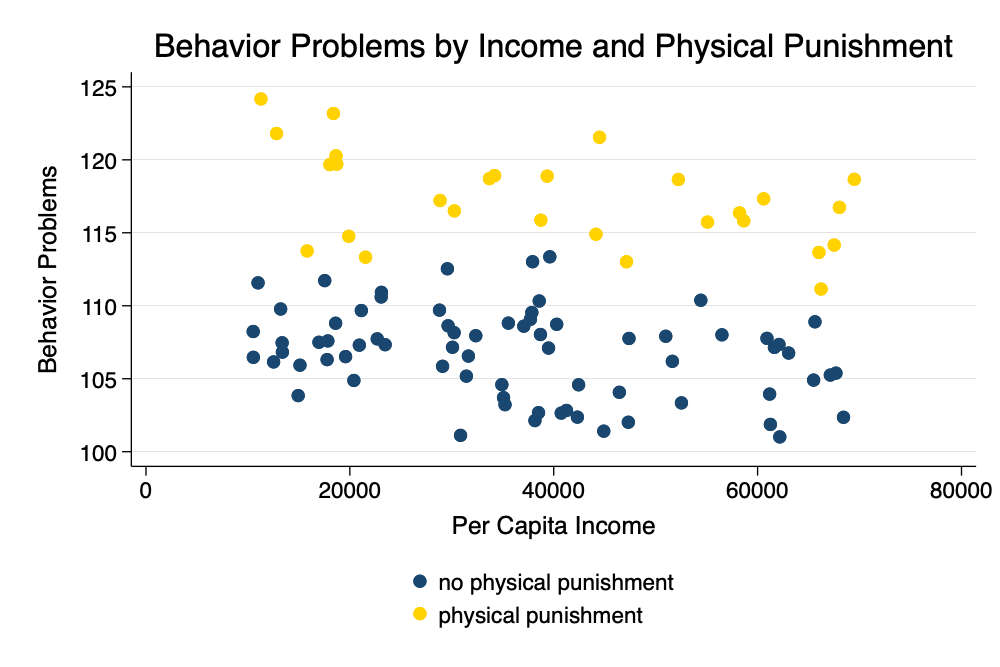
Consider a cross-national data set where we are attempting to
understand predictors of behavior problems as a function of
per capita income and parental use of physical
punishment.
Simulate Some Data
. clear all
. set obs 100
Number of observations (_N) was 0, now 100.
. generate income = runiform(10000, 70000)
. generate physical_punishment = rbinomial(1,.3)
. generate country = int(_n/10) + 1
. generate e = rnormal(0,1) // individual error
. generate u = country - 5 // random intercept
. generate behavior_problems = 110 + -.0001 * income + 10 * physical_punishment
>  + u + e // plausible regression relationship
. twoway (scatter behavior_problems income if physical_punishment ==0) ///
> (scatter behavior_problems income if physical_punishment == 1), ///
> legend(order(1 "no physical punishment" 2 "physical punishment") pos(6)) ///
> title("Behavior Problems by Income and Physical Punishment") ///
> xtitle("Per Capita Income") ///
> ytitle("Behavior Problems") ///
> scheme(michigan)
. graph export myscatter.png, width(1000) replace
file
    /Users/agrogan/Desktop/GitHub/multilevel/centering-in-cross-sectional-dat
    > a/myscatter.png saved as PNG format
Scatterplot
Multilevel Model
. mixed behavior_problems income physical_punishment || country:

Performing EM optimization ...

Performing gradient-based optimization:
Iteration 0:  Log likelihood = -157.07646
Iteration 1:  Log likelihood = -157.07646

Computing standard errors ...

Mixed-effects ML regression                         Number of obs    =     100
Group variable: country                             Number of groups =      11
                                                    Obs per group:
                                                                 min =       1
                                                                 avg =     9.1
                                                                 max =      10
                                                    Wald chi2(2)     = 2230.63
Log likelihood = -157.07646                         Prob > chi2      =  0.0000

─────────────┬────────────────────────────────────────────────────────────────
behavior_p~s │ Coefficient  Std. err.      z    P>|z|     [95% conf. interval]
─────────────┼────────────────────────────────────────────────────────────────
      income │  -.0001021   5.25e-06   -19.44   0.000    -.0001124   -.0000918
physical_p~t │   9.859842   .2315382    42.58   0.000     9.406036    10.31365
       _cons │   110.9004   .9343151   118.70   0.000     109.0691    112.7316
─────────────┴────────────────────────────────────────────────────────────────

─────────────────────────────┬────────────────────────────────────────────────
  Random-effects parameters  │   Estimate   Std. err.     [95% conf. interval]
─────────────────────────────┼────────────────────────────────────────────────
country: Identity            │
                  var(_cons) │   8.878869   3.878162      3.771943    20.90019
─────────────────────────────┼────────────────────────────────────────────────
               var(Residual) │   .8283655   .1242951      .6173058    1.111587
─────────────────────────────┴────────────────────────────────────────────────
LR test vs. linear model: chibar2(01) = 183.09        Prob >= chibar2 = 0.0000
We note that -1.021 is the effect of every additional $10,000 of per
capita income. 9.860 is the effect of physical punishment.
Notably, for this handout, 110.900 is the level of behavior problems
for a child who did not receive physical punishment living in a
family with $0income.
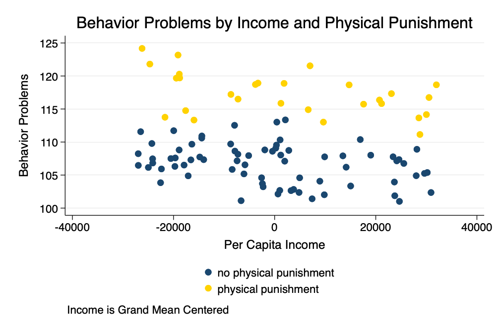
Grand Mean Centering
Grand mean centering helps us to have more meaningful intercepts of
our continuous variables.
Essentially, we are going to create \(\text{income}_{\text{grand mean centered}} =
\text{income} - \overline{\text{income}}\)
. egen m_income = mean(income) // grand mean of income
. generate c_income = income - m_income // grand mean centered income
. twoway (scatter behavior_problems c_income if physical_punishment ==0) ///
> (scatter behavior_problems c_income if physical_punishment == 1), ///
> legend(order(1 "no physical punishment" 2 "physical punishment") pos(6)) ///
> title("Behavior Problems by Income and Physical Punishment") ///
> caption("Income is Grand Mean Centered") ///
> xtitle("Per Capita Income") ///
> ytitle("Behavior Problems") ///
> scheme(michigan)
. graph export myscatter2.png, width(1000) replace
file
    /Users/agrogan/Desktop/GitHub/multilevel/centering-in-cross-sectional-dat
    > a/myscatter2.png saved as PNG format
Scatterplot With Grand Mean
Centering
In a graph, we see that grand mean centering has transformed
the intercept so now the \(\beta_0\)
term is the level of behavior problems for the average child
who did not recieve physical punishment.
Multilevel Model
. mixed behavior_problems c_income physical_punishment || country:

Performing EM optimization ...

Performing gradient-based optimization:
Iteration 0:  Log likelihood = -157.07646
Iteration 1:  Log likelihood = -157.07646

Computing standard errors ...

Mixed-effects ML regression                         Number of obs    =     100
Group variable: country                             Number of groups =      11
                                                    Obs per group:
                                                                 min =       1
                                                                 avg =     9.1
                                                                 max =      10
                                                    Wald chi2(2)     = 2230.63
Log likelihood = -157.07646                         Prob > chi2      =  0.0000

─────────────┬────────────────────────────────────────────────────────────────
behavior_p~s │ Coefficient  Std. err.      z    P>|z|     [95% conf. interval]
─────────────┼────────────────────────────────────────────────────────────────
    c_income │  -.0001021   5.25e-06   -19.44   0.000    -.0001124   -.0000918
physical_p~t │   9.859842   .2315382    42.58   0.000     9.406036    10.31365
       _cons │   106.7117   .9085729   117.45   0.000      104.931    108.4925
─────────────┴────────────────────────────────────────────────────────────────

─────────────────────────────┬────────────────────────────────────────────────
  Random-effects parameters  │   Estimate   Std. err.     [95% conf. interval]
─────────────────────────────┼────────────────────────────────────────────────
country: Identity            │
                  var(_cons) │   8.878869   3.878162      3.771942    20.90019
─────────────────────────────┼────────────────────────────────────────────────
               var(Residual) │   .8283655   .1242951      .6173058    1.111588
─────────────────────────────┴────────────────────────────────────────────────
LR test vs. linear model: chibar2(01) = 183.09        Prob >= chibar2 = 0.0000
We see that the \(\beta_1\) and
\(\beta_2\) regression coefficients
have not changed. However, the intercept, \(\beta_0\) has changed, and is now more
meaningful.
Group Mean Centering
In group mean centering, we are doing something slightly different.
We are creating a mean for each group, which in this data is
country: e.g. \(\text{income}_{\text{group mean centered}} =
\text{income} - \overline{\text{income}}_{.j}\), where \(j\) is the index for group or
country.
. bysort country: egen m_g_income = mean(income) // GROUP mean of income
. generate c_g_income = income - m_g_income // GROUP mean centered income
. bysort country: egen m_g_physical_punishment = mean(physical_punishment) // G
> ROUP mean of physical punishment
. generate c_g_physical_punishment = physical_punishment - m_g_physical_punishm
> ent // GROUP mean centered physical punishment
Interestingly, group mean centering has many implications.
Here I focus on how employing different variables might provide
conceptually or theoretically different results. For
the sake of parismony, in the brief discussion below I focus on these
conceptual or theoretical differences, and do not
provide output. I use the quietly prefix to suppress
output.
Equation
Two versions of the equation are equally appropriate. Both address
conceptually or theoretically different questions.
Covariate and Group Mean
One parameterization of the multilevel model is to enter the
covariate and its group level mean i.e. \(x_{ij}\) and \(\overline{x_{.j}}\).
A second, equally valid, but conceptually different parameterization
of the multilevel model is to enter the covariate deviated from its
group level mean and the group level mean i.e. \(x_{ij} - \overline{x_{.j}}\) and \(\overline{x_{.j}}\).
This second parameterization focuses on how individuals differ
from their country level means, and country level
means.
What is the effect of income deviated from its country level
mean, country level mean income, physical punishment
deviated from its country level punishment, and country level
mean of physical punishment on behavior problems?