https://ec.europa.eu/jrc/en/research-topic/forestry/qr-tree-project/norway-spruce

Data Source

The data used in this example are derived from the R package Functions and Datasets for “Forest Analytics with R”.

According to the documentation, the source of these data are: “von Guttenberg’s Norway spruce (Picea abies [L.] Karst) tree measurement data.”

The documentation goes on to further note that:

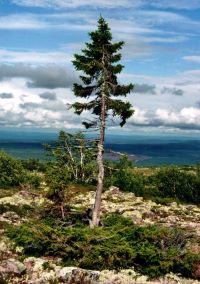
“The data are measures from 107 trees. The trees were selected as being of average size from healthy and well stocked stands in the Alps.”

.     use gutten.dta, clear

Variables

site Growth quality class of the tree’s habitat. 5 levels.

location Distinguishes tree location. 7 levels.

tree An identifier for the tree within location.

age.base The tree age taken at ground level.

It might be best to use a centered age variable, centered at the grand mean of tree age:

. egen ageMEAN = mean(age_base)

. generate ageCENTERED = age_base - ageMEAN

height Tree height, m.

dbh.cm Tree diameter, cm.

volume Tree volume.

age.bh Tree age taken at 1.3 m.

tree.ID A factor uniquely identifying the tree.

Calculating \(R^2\)

Roberts et al. (2015) explain that there are multiple competing perspectives, and formulas, for calculating an estimate of \(R^2\) for multilevel models.

Here we adopt an approach advanced by Cox (link below).

Outline

1. Estimate MLM: mixed y x1 x2 x3 || id:
2. Generate predicted values: predict yhat
3. Estimate correlation of observed and predicted: corr y yhat
4. Then square this correlation: \(R^2 = r^2\)

Estimate MLM

. mixed height age_base site i.location || tree_ID:

Performing EM optimization: 

Performing gradient-based optimization: 

Iteration 0:   log likelihood = -3050.2621  
Iteration 1:   log likelihood = -3050.2621  

Computing standard errors:

Mixed-effects ML regression                     Number of obs     =      1,200
Group variable: tree_ID                         Number of groups  =        107

                                                Obs per group:
                                                              min =          5
                                                              avg =       11.2
                                                              max =         15

                                                Wald chi2(8)      =    8663.47
Log likelihood = -3050.2621                     Prob > chi2       =     0.0000

─────────────┬────────────────────────────────────────────────────────────────
      height │      Coef.   Std. Err.      z    P>|z|     [95% Conf. Interval]
─────────────┼────────────────────────────────────────────────────────────────
    age_base │   .2143496   .0023831    89.95   0.000     .2096789    .2190203
        site │  -3.866312   .1608021   -24.04   0.000    -4.181478   -3.551145
             │
    location │
          2  │  -.5436647   1.247694    -0.44   0.663    -2.989099     1.90177
          3  │   .5090705   .6487789     0.78   0.433    -.7625129    1.780654
          4  │   .0954239   .7056685     0.14   0.892    -1.287661    1.478509
          5  │  -.0590126   .5182994    -0.11   0.909    -1.074861    .9568356
          6  │   .2078246   .6884815     0.30   0.763    -1.141574    1.557224
          7  │  -1.210496   .7524348    -1.61   0.108    -2.685241    .2642491
             │
       _cons │   12.27241   .5513051    22.26   0.000     11.19187    13.35294
─────────────┴────────────────────────────────────────────────────────────────

─────────────────────────────┬────────────────────────────────────────────────
  Random-effects Parameters  │   Estimate   Std. Err.     [95% Conf. Interval]
─────────────────────────────┼────────────────────────────────────────────────
tree_ID: Identity            │
                  var(_cons) │   2.106718   .3939037      1.460337    3.039204
─────────────────────────────┼────────────────────────────────────────────────
               var(Residual) │   8.397623       .359      7.722667    9.131569
─────────────────────────────┴────────────────────────────────────────────────
LR test vs. linear model: chibar2(01) = 127.84        Prob >= chibar2 = 0.0000

Predict \(\hat{y}\)

. predict yhat if e(sample) // calculate predicted values
(option xb assumed)

Estimate Correlation of \(y\) and \(\hat{y}\)

We then obtain the correlation of y and \(\hat{y}\), the observed and predicted values.

. corr height yhat 
(obs=1,200)

             │   height     yhat
─────────────┼──────────────────
      height │   1.0000
        yhat │   0.9364   1.0000

So our estimate for \(R^2\) is .93636423 squared, or .87677798.

References

Cox, N. J. (n.d.). Stata FAQ: Do-it-yourself R-squared. Retrieved May 7, 2020, from https://www.stata.com/support/faqs/statistics/r-squared/

Roberts, J. K., Monaco, J. P., Stovall, H., & Foster, V. (2015). Explained Variance in Multilevel Models. In Handbook of Advanced Multilevel Analysis. https://doi.org/10.4324/9780203848852.ch12