Multilevel Structure

Structure of the data may be different at different levels. Results may differ greatly when we apply multilevel thinking.

Author

Affiliation

Andy Grogan-Kaylor

University of Michigan

1 Introduction

Associations between two variables can be very different (or even reversed) depending upon whether or not the analysis is “aware” of the grouped, nested, or clustered nature of the data (Nieuwenhuis 2015). In multilevel analysis, the groups are often neighborhoods, communities, or even different countries.

A model that is “aware” of the clustered nature of the data may provide very different–likely better–substantive conclusions than a model that is not aware of the clustered nature of the data. This phenomena is closely related to the “ecological fallacy”: the idea that group level and individual level relationships are not necessarily the same (Firebaugh 2001).

2 Set a Random Seed For Replicability

set.seed(1080) # random seed

3 Call The Libraries

library(ggplot2) # beautiful graphs

library(lme4) # MLM

library(sjPlot) # nice tables for MLM

4 Simulate Some Data

e <- rnorm(10, 0, 1) # error

# group 1

group1 <- rep(1, 10)

x1 <- seq(1, 10)

y1 <- 50 + 1 * x1 + e

# group 2

group2 <- rep(2, 10)

x2 <- seq(11, 20)

y2 <- 30 + 1 * x2 + e

# group 3

group3 <- rep(3, 10)

x3 <- seq(21, 30)

y3 <- 10 + 1 * x3 + e

# combine into a dataframe

x <- c(x1, x2, x3)

y <- c(y1, y2, y3)

group <- factor(c(group1, group2, group3))

multilevelstructure <- data.frame(x, y, group) 

5 Graphs

5.1 A “Naive” Graph

This “naive” graph is unaware of the grouped nature of the data.

library(ggplot2)

p0 <- ggplot(multilevelstructure, 
             aes(x = x,
                 y = y)) +
  geom_smooth(method = "lm") +
  labs(title = "y as a function of x") +
  theme_minimal()

p0 + geom_point() # replay and add points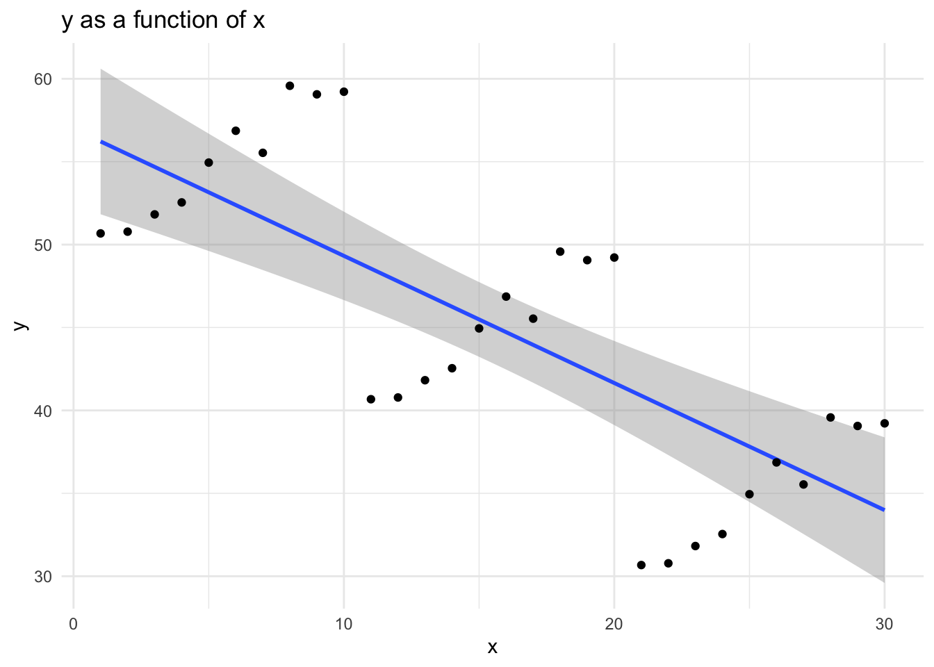

5.2 An “Aware” Graph

This “aware” graph is aware of the grouped nature of the data.

p0 + 
  geom_point(aes(color = group)) + # points with group color
  geom_smooth(aes(color = group), # smoothers with group color
              method = "lm") + 
  scale_color_viridis_d()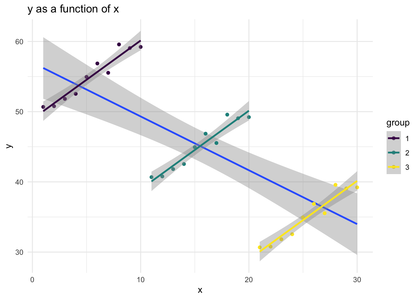

6 Regressions

6.1 A “Naive” OLS Analysis

The OLS model with only x as a covariate is not aware of the grouped structure of the data, and the coefficient for x reflects this.

myOLS <- lm(y ~ x, data = multilevelstructure)

sjPlot::tab_model(myOLS,
                  show.se = TRUE,
                  show.ci = FALSE,
                  show.stat = TRUE)

	y
Predictors	Estimates	std. Error	Statistic	p
(Intercept)	56.99	2.25	25.29	<0.001
x	-0.77	0.13	-6.04	<0.001
Observations	30
R2 / R2 adjusted	0.566 / 0.550

6.2 An “Aware” MLM Analysis

The multilevel model is aware of the grouped structure of the data, and the coefficient for x reflects this.

myMLM <- lmer(y ~ x + (1 | group), data = multilevelstructure)

sjPlot::tab_model(myMLM,
                  show.se = TRUE,
                  show.ci = FALSE,
                  show.stat = TRUE)

	y
Predictors	Estimates	std. Error	Statistic	p
(Intercept)	27.82	12.25	2.27	0.032
x	1.11	0.06	17.87	<0.001
Random Effects
σ2	0.96
τ00 group	447.52
ICC	1.00
N group	3
Observations	30
Marginal R2 / Conditional R2	0.177 / 0.998

7 A Thought Experiment

When might a situation like this arise in practice? This is surprisingly difficult to think through.

Imagine that x is a protective factor, or an intervention or treatment. Imagine that y is a desirable outcome, like improved mental health or psychological well being.

Now imagine that community members provide more of the protective factor or more of the intervention in communities where there are lower levels of the desirable outcome. If we think about it, this is a very plausible situation.

A Naive Analysis Would Misconstrue The Results

A naive analysis that was unaware of the grouped nature of the data would therefore misconstrue the results, suggesting that the intervention was harmful, when it was in fact helpful.

p0 + 
  geom_point(aes(color = group)) + # points with group color
  geom_smooth(aes(color = group), # smoothers with group color
              method = "lm") + 
  labs(title = "psychological well-being as a function of intervention or treatment",
       x = "intervention or treatment",
       y = "psychological well-being") +
  scale_color_viridis_d()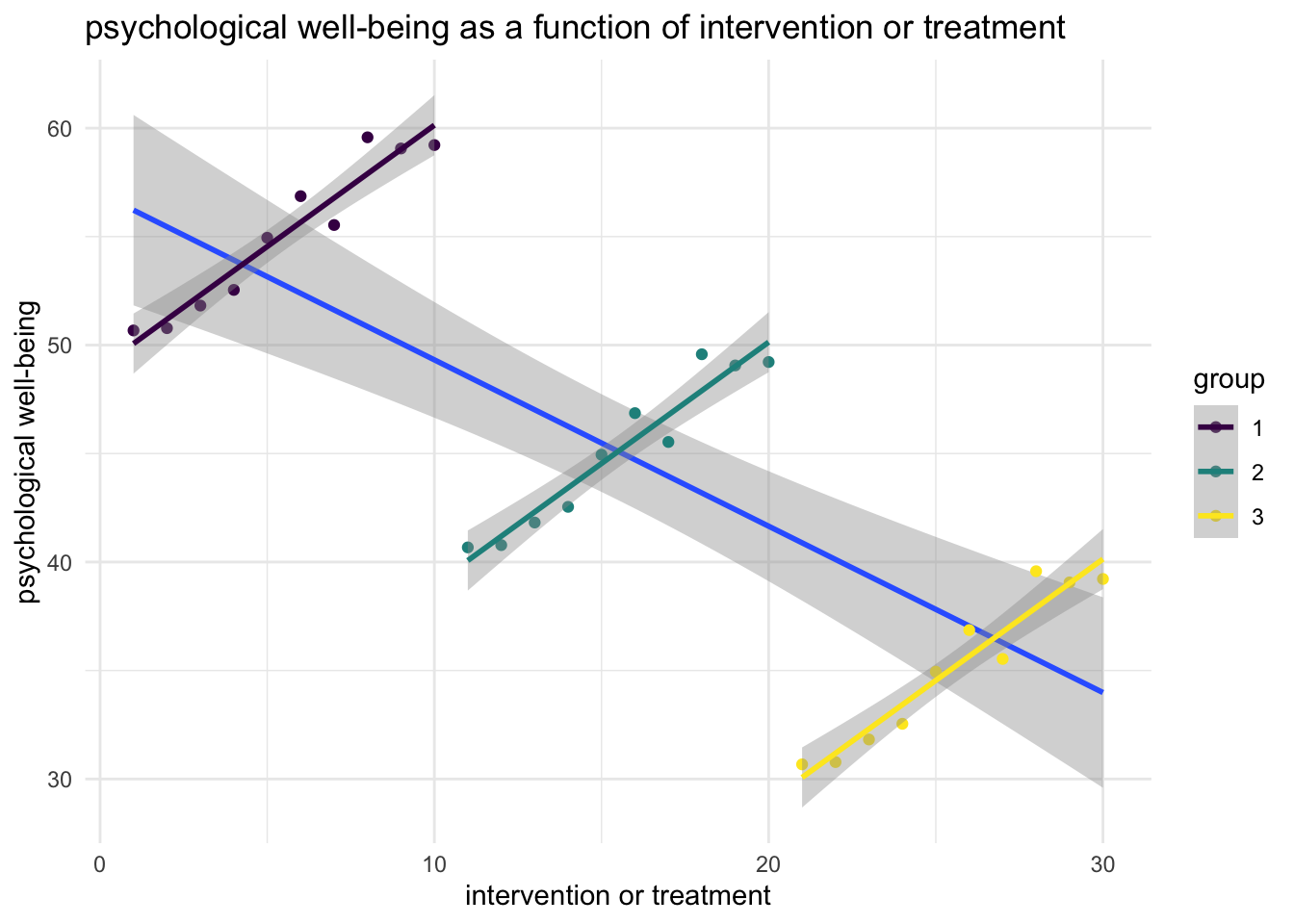

These data are constructed to provide this kind of extreme example, but it easy to see how multilevel thinking, and multilevel analysis may provide better answers than we would get if we ignored the grouped nature of the data.

References

Firebaugh, G. 2001. “Ecological Fallacy, Statistics Of.” In International Encyclopedia of the Social & Behavioral Sciences, edited by Neil J. Smelser and Paul B. Baltes, 4023–26. Oxford: Pergamon. https://doi.org/https://doi.org/10.1016/B0-08-043076-7/00765-8.

Nieuwenhuis, Rense. 2015. “Association, Aggregation, and Paradoxes: On the Positive Correlation Between Fertility and Women’s Employment.” Demographic Research 32 (March). https://www.demographic-research.org/volumes/vol32/23/.