The Count

The Count and Friends
Andy Grogan-Kaylor
Andy Grogan-Kaylor
16 Oct 2021
\(F(y) = \beta_0 + \beta_1 x_1 + ...\)
\(y = \ln(count): 1, 2, 3, \text{etc.}\)
Think about IRR’s, predicted counts, non-linearity
So much of categorical data analysis depends upon arguments for “functional form”. When do we think these arguments are valid?

The Count and Friends
From the Stata documentation:
“Poisson regression fits models of the number of occurrences (counts) of an event. The Poisson distribution has been applied to diverse events, such as the number of soldiers kicked to death by horses in the Prussian army (von Bortkiewicz 1898); the pattern of hits by buzz bombs launched against London during World War II (Clarke 1946); telephone connections to a wrong number (Thorndike 1926); and disease incidence, typically with respect to time, but occasionally with respect to space.”
The Poisson distribution is a modified form of the binomial distribution that is useful for the analysis of phenomena characterized by discrete, rare events. For example, in a study of the distribution of a rare plant among a number of quadrats, a majority of plots may contain no specimens, a smaller number a single plant, and still smaller numbers two, three, or more plants. If a single plant per quadrat is expected, the mean µ = 1 and the “0” and “1” classes occur at 37% each, the “2” class at 18%, the “3” class at 6%, and larger classes take up the remaining 2%. The characteristic test for a Poisson is that the variance equals the mean, which in the plant example means that the rare plant is randomly distributed. Note, that, In the distributions above, as the mean \(\mu\) increases towards 10, the distribution approaches normality.
The Poisson may be used to evaluate whether events occur independently in time as well as space. In a classic example, Bortkiewicz (1898) studied the distribution of 122 men kicked to death by horses among ten Prussian army corps over 20 years. In most years in most corps, no one dies from being kicked; in one corp in one year, four men were kicked to death. Does this mean something was amiss in this particular corp? Analysis indicates that the observed frequencies conform quite closely to the expected Poisson frequencies, and that the mean and variance are almost identical, as expected. The corp was just “unlucky” in the sense that it is in the extreme tail of an ordinary run of events.
http://www.mun.ca/biology/scarr/smcPoisson_distributions.html
Normal distribution:
\[ P(x) = \frac{1}{\sigma \sqrt{2 \pi}} e^{-(x-\mu)^2/(2 \sigma^2)} \]
Standardized Normal Distribution:
\[ P(z) = \frac{1}{\sqrt{2 \pi}} e^{-z^2/2} \]
2 parameters:
\[ x \sim N(\mu,\sigma) \]
. histogram x, title("Normally Distributed Random Variable") scheme(michigan)
(bin=29, start=-3.0031285, width=.20304677)
. graph export myhistogram.png, width(500) replace
file /Users/agrogan/Desktop/GitHub/newstuff/categorical/count-regression/myhistogram.png saved as
PNG format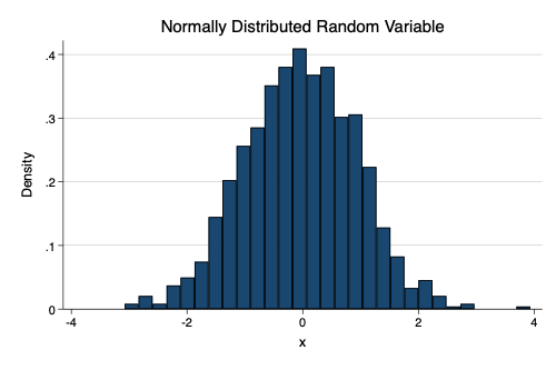
histogram of random normal variable
\[ P(Y=y) = e^{-\lambda} \frac{\lambda^y}{y!} \]
A Poisson with large lambda looks very similar to a normal distribution.
. histogram w, title("Poisson Distributed Random Variable") scheme(michigan)
(bin=29, start=0, width=.13793103)
. graph export myhistogram2.png, width(500) replace
file /Users/agrogan/Desktop/GitHub/newstuff/categorical/count-regression/myhistogram2.png saved
as PNG format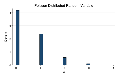
histogram of random Poisson variable
\[ x \sim Poisson(\lambda) \]
\(\lambda\) is both mean and variance.
. expand mycount // create individual observations
(9 zero counts ignored; observations not deleted)
(7 observations created)
. twoway scatter y x, ///
> by(field, title("Randomly Located Ducks")) ///
> mlab(mylabel) mlabsize(vlarge) ///
> msymbol(none) ///
> legend(order(1 "🦆 Duck")) ///
> scheme(michigan) plotr(fcolor(olive_teal)). graph export ducks.png, width(1000) replace
file /Users/agrogan/Desktop/GitHub/newstuff/categorical/count-regression/ducks.png saved as PNG
format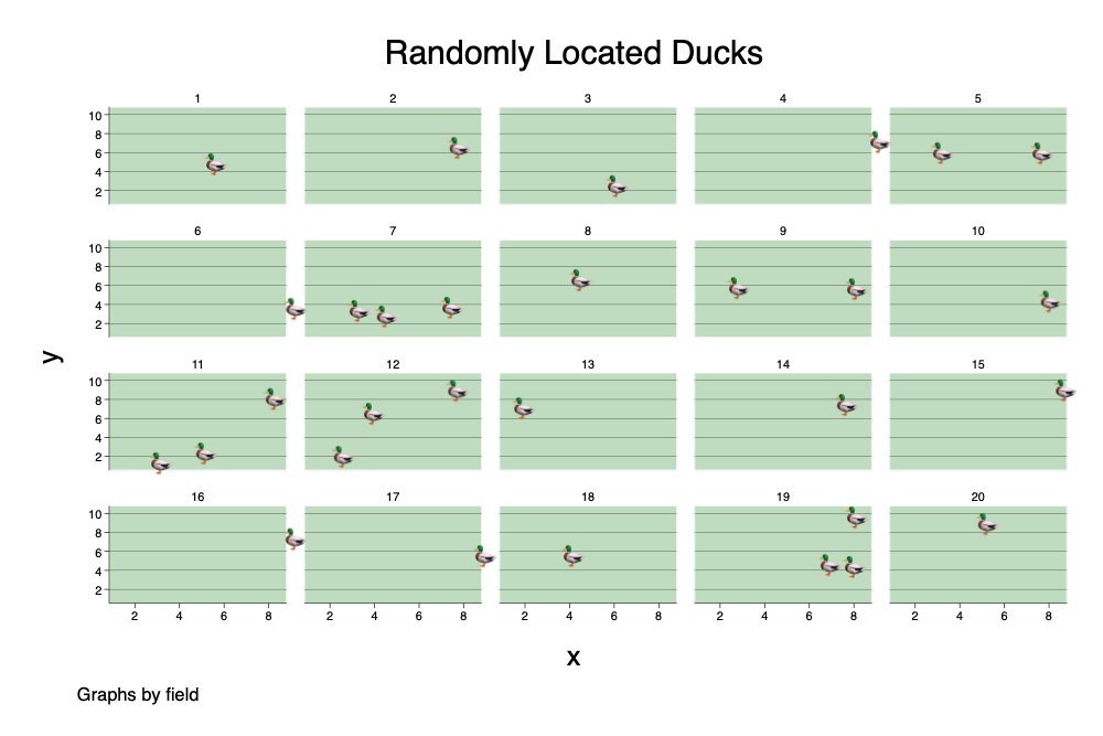
Randomly Located Ducks
. twoway scatter y2 t, ///
> by(timeperiod, title("Forest Fires At Random Times", size(vhuge)) cols(10)) ///
> ytitle("", size(zero)) ylabel(none) xtitle("", size(zero)) xlabel(none) ///
> subtitle(, size(vhuge)) ///
> mlab(mylabel2) mlabsize(vhuge) ///
> msymbol(none)  ///
> legend(order(1 "🔥 Forest Fire")) ///
> scheme(michigan) plotr(fcolor(gs14)) ///
> xsize(5) ysize(1)
. graph export fires.png, width(1000) replace
file /Users/agrogan/Desktop/GitHub/newstuff/categorical/count-regression/fires.png saved as PNG
format
Forest Fires At Random Times
The data are an extract of the National Survey of Children’s Health, 2018. The data contain information on children’s exposure to various Adverse Childhood Experiences (ACEs) and their demographic characteristics.
. describe

Contains data from ../predict-and-margins-substantive-example/NSCH_ACES.dta
 Observations:        30,530
    Variables:            23                  20 Oct 2020 14:50
───────────────────────────────────────────────────────────────────────────────────────────────────
Variable      Storage   Display    Value
    name         type    format    label      Variable label
───────────────────────────────────────────────────────────────────────────────────────────────────
sc_sex          byte    %30.0g     sc_sex_lab
                                              Sex of Selected Child
ace3            byte    %30.0g     ace3_lab   Child Experienced - Parent or Guardian Divorced
ace4            byte    %30.0g     ace4_lab   Child Experienced - Parent or Guardian Died
ace5            byte    %30.0g     ace5_lab   Child Experienced - Parent or Guardian Time in Jail
ace6            byte    %30.0g     ace6_lab   Child Experienced - Adults Slap, Hit, Kick, Punch
                                                Others
ace7            byte    %30.0g     ace7_lab   Child Experienced - Victim of Violence
ace8            byte    %30.0g     ace8_lab   Child Experienced - Lived with Mentally Ill
ace9            byte    %30.0g     ace9_lab   Child Experienced - Lived with Person with
                                                Alcohol/Drug Problem
ace10           byte    %30.0g     ace10_lab
                                              Child Experienced - Treated Unfairly Because of Race
ace1            byte    %30.0g     ace1_lab   Hard to Cover Basics Like Food or Housing
sc_race_r       byte    %48.0g     sc_race_r_lab
                                              Race of Selected Child, Detailed
sc_racer        byte    %31.0g     sc_racer_lab
                                              Race of Selected Child, Recode
higrade         byte    %61.0g     higrade_lab
                                              Highest Level of Education among Reported Adults
depress         byte    %9.0g                 RECODE of k2q32b (Depression Currently)
ace1R           byte    %9.0g                 RECODE of ace1 (Hard to Cover Basics Like Food or
                                                Housing)
ace3R           byte    %9.0g                 RECODE of ace3 (Child Experienced - Parent or
                                                Guardian Divorced)
ace4R           byte    %9.0g                 RECODE of ace4 (Child Experienced - Parent or
                                                Guardian Died)
ace5R           byte    %9.0g                 RECODE of ace5 (Child Experienced - Parent or
                                                Guardian Time in Jail)
ace6R           byte    %9.0g                 RECODE of ace6 (Child Experienced - Adults Slap, Hit,
                                                Kick, Punch Others)
ace7R           byte    %9.0g                 RECODE of ace7 (Child Experienced - Victim of
                                                Violence)
ace8R           byte    %9.0g                 RECODE of ace8 (Child Experienced - Lived with
                                                Mentally Ill)
ace9R           byte    %9.0g                 RECODE of ace9 (Child Experienced - Lived with Person
                                                with Alcohol/Drug Problem)
ace10R          byte    %9.0g                 RECODE of ace10 (Child Experienced - Treated Unfairly
                                                Because of Race)
───────────────────────────────────────────────────────────────────────────────────────────────────
Sorted by: . graph export myhistogram3.png, width(1000) replace
file /Users/agrogan/Desktop/GitHub/newstuff/categorical/count-regression/myhistogram3.png saved
as PNG format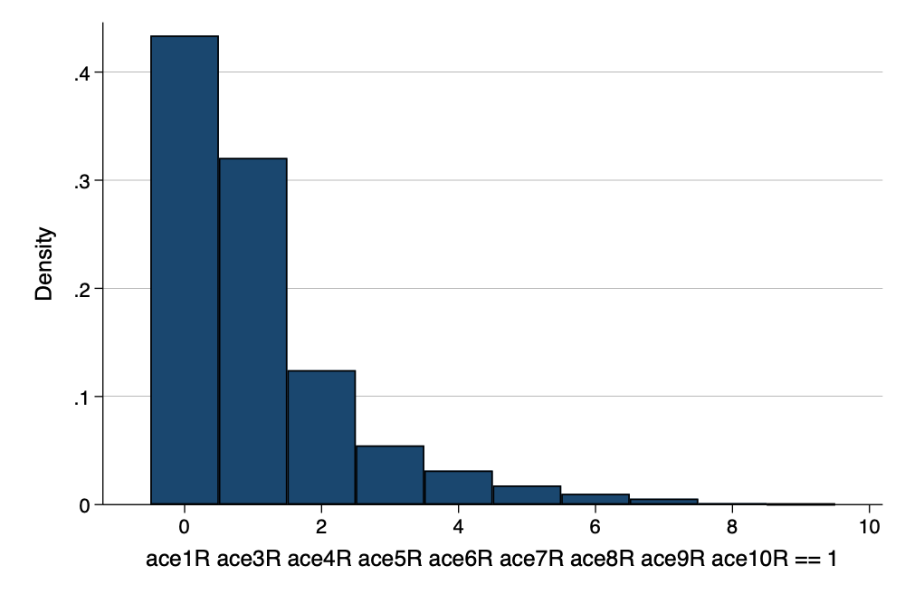
Count of ACEs
. poisson acecount sc_sex i.sc_race_r i.higrade

Iteration 0:   log likelihood = -44759.253
Iteration 1:   log likelihood = -44758.999
Iteration 2:   log likelihood = -44758.999

Poisson regression                                     Number of obs =  30,530
                                                       LR chi2(9)    = 2054.20
                                                       Prob > chi2   =  0.0000
Log likelihood = -44758.999                            Pseudo R2     =  0.0224

─────────────────────────────────┬────────────────────────────────────────────────────────────────
                        acecount │ Coefficient  Std. err.      z    P>|z|     [95% conf. interval]
─────────────────────────────────┼────────────────────────────────────────────────────────────────
                          sc_sex │   -.012823   .0111291    -1.15   0.249    -.0346357    .0089897
                                 │
                       sc_race_r │
Black or African American alone  │   .2662761   .0196921    13.52   0.000     .2276802    .3048719
American Indian or Alaska Nat..  │   .5971063   .0447201    13.35   0.000     .5094566     .684756
                    Asian alone  │  -.6243821   .0358521   -17.42   0.000    -.6946509   -.5541134
Native Hawaiian and Other Pac..  │   .2067409   .0969415     2.13   0.033     .0167392    .3967427
          Some Other Race alone  │   .0675521   .0324881     2.08   0.038     .0038765    .1312277
              Two or More Races  │   .2818125   .0190548    14.79   0.000     .2444658    .3191593
                                 │
                         higrade │
High school (including vocat..)  │   .0632486   .0322397     1.96   0.050       .00006    .1264372
          More than high school  │  -.3786108    .030587   -12.38   0.000    -.4385602   -.3186615
                                 │
                           _cons │   .3399425   .0345283     9.85   0.000     .2722683    .4076166
─────────────────────────────────┴────────────────────────────────────────────────────────────────. poisson, irr
Poisson regression Number of obs = 30,530
LR chi2(9) = 2054.20
Prob > chi2 = 0.0000
Log likelihood = -44758.999 Pseudo R2 = 0.0224
─────────────────────────────────┬────────────────────────────────────────────────────────────────
acecount │ IRR Std. err. z P>|z| [95% conf. interval]
─────────────────────────────────┼────────────────────────────────────────────────────────────────
sc_sex │ .9872589 .0109873 -1.15 0.249 .9659573 1.00903
│
sc_race_r │
Black or African American alone │ 1.305095 .0257001 13.52 0.000 1.255684 1.356451
American Indian or Alaska Nat.. │ 1.816854 .0812498 13.35 0.000 1.664386 1.983288
Asian alone │ .5355922 .0192021 -17.42 0.000 .4992487 .5745815
Native Hawaiian and Other Pac.. │ 1.229664 .1192054 2.13 0.033 1.01688 1.486973
Some Other Race alone │ 1.069886 .0347586 2.08 0.038 1.003884 1.140227
Two or More Races │ 1.32553 .0252577 14.79 0.000 1.276939 1.37597
│
higrade │
High school (including vocat..) │ 1.065292 .0343446 1.96 0.050 1.00006 1.134778
More than high school │ .6848121 .0209463 -12.38 0.000 .6449644 .7271216
│
_cons │ 1.404867 .0485076 9.85 0.000 1.312939 1.503231
─────────────────────────────────┴────────────────────────────────────────────────────────────────
Note: _cons estimates baseline incidence rate.Due to population heterogeneity (diversity, variation), variance may be \(>\) mean. This is often empirically the case.
\[ \text{var}(y) > \text{mean}(y) \]
\[ y \sim Poisson(\mu) \]
\[ \ln(\mu) = \beta_0 + \beta_1 x + \text{offset} + \text{dispersion} + etc. \]
. nbreg acecount sc_sex i.sc_race_r i.higrade, irr

Fitting Poisson model:

Iteration 0:   log likelihood = -44759.253
Iteration 1:   log likelihood = -44758.999
Iteration 2:   log likelihood = -44758.999

Fitting constant-only model:

Iteration 0:   log likelihood =   -43591.3
Iteration 1:   log likelihood = -43392.427
Iteration 2:   log likelihood = -43391.748
Iteration 3:   log likelihood = -43391.748

Fitting full model:

Iteration 0:   log likelihood = -42801.127
Iteration 1:   log likelihood = -42775.936
Iteration 2:   log likelihood = -42775.864
Iteration 3:   log likelihood = -42775.864

Negative binomial regression                           Number of obs =  30,530
                                                       LR chi2(9)    = 1231.77
Dispersion: mean                                       Prob > chi2   =  0.0000
Log likelihood = -42775.864                            Pseudo R2     =  0.0142

─────────────────────────────────┬────────────────────────────────────────────────────────────────
                        acecount │        IRR   Std. err.      z    P>|z|     [95% conf. interval]
─────────────────────────────────┼────────────────────────────────────────────────────────────────
                          sc_sex │   .9873253   .0140708    -0.90   0.371     .9601287    1.015292
                                 │
                       sc_race_r │
Black or African American alone  │   1.326253   .0350126    10.70   0.000     1.259374    1.396682
American Indian or Alaska Nat..  │   1.864104   .1222717     9.49   0.000     1.639221    2.119839
                    Asian alone  │   .5378757   .0222161   -15.01   0.000     .4960489    .5832294
Native Hawaiian and Other Pac..  │   1.244574   .1624972     1.68   0.094     .9635716    1.607524
          Some Other Race alone  │   1.083969   .0459946     1.90   0.057     .9974679    1.177971
              Two or More Races  │   1.325755   .0336113    11.12   0.000     1.261488    1.393296
                                 │
                         higrade │
High school (including vocat..)  │    1.06806   .0468996     1.50   0.134      .979983    1.164053
          More than high school  │   .6831897   .0282212    -9.22   0.000     .6300572     .740803
                                 │
                           _cons │   1.403757   .0647737     7.35   0.000     1.282374    1.536629
─────────────────────────────────┼────────────────────────────────────────────────────────────────
                        /lnalpha │  -.5443067   .0239625                     -.5912723   -.4973411
─────────────────────────────────┼────────────────────────────────────────────────────────────────
                           alpha │   .5802439   .0139041                      .5536224    .6081455
─────────────────────────────────┴────────────────────────────────────────────────────────────────
Note: Estimates are transformed only in the first equation to incidence-rate ratios.
Note: _cons estimates baseline incidence rate.
LR test of alpha=0: chibar2(01) = 3966.27 Prob >= chibar2 = 0.000. graph export myyhats.png, width(1000) replace
file /Users/agrogan/Desktop/GitHub/newstuff/categorical/count-regression/myyhats.png saved as PNG
format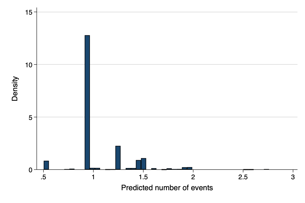
Predicted Count of ACEs
In some data sets, we will have a years exposed or time exposed variable. It is important to control for this variable.