Interactions in Logistic Regression

Author

Andy Grogan-Kaylor

Published

April 25, 2024

1 Background

The purpose of this tutorial is to illustrate the idea that in logistic regression, the \(\beta\) parameter for an interaction term may not accurately characterize the underlying interactive relationships.

This idea may be easier to describe if we recall the formula for a logistic regression:

\[\ln\left(\frac{P(y)}{1 - P(y)}\right) = \beta_0 + \beta_1 x_1 + \beta_2 x_2 + \beta_3 x_1 \times x_2 \tag{1}\]

Warning

In the above formula, the sign, and statistical significance, of \(\beta_3\) may not accurately characterize the underlying relationship.

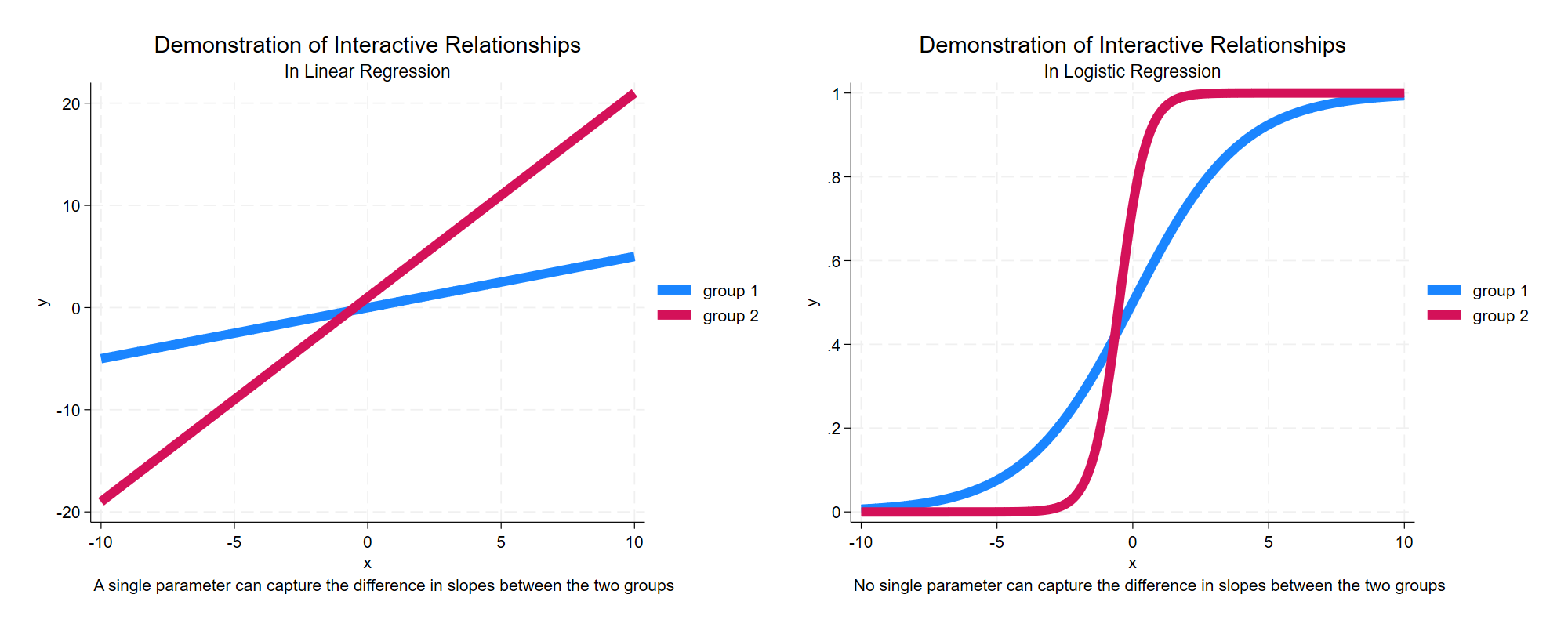
Demonstration of Interactive Relationships

Key Idea

In a linear model, a single parameter can capture the difference in slopes between the two groups. In a non-linear model, no single parameter can capture the difference in slopes between the two groups.

Some Calculus (Not Essential To The Discussion)

Imagine a linear model:

\[y = \beta_0 + \beta_1 x_1 + \beta_2 x_2 + \beta_3 x_1 \times x_2 + e_i\]

Here (following (Ai and Norton 2003)):

\[\frac{\partial y}{\partial x_1 \partial x_2} = \beta_3\]

We use \(\text{logit}\) to describe:

\[\ln\left(\frac{P(y)}{1 - P(y)}\right)\]

In the logistic model, the quantity:

\[\frac{\partial \text{logit} (y)}{\partial x_1 \partial x_2}\]

does not have such a straightforward solution, and–importantly for this discussion–is not simply equal to \(\beta_3\).

2 Get The Data

We start by obtaining simulated data from StataCorp.


clear all

graph close _all

use http://www.stata-press.com/data/r15/margex, clear

(Artificial data for margins)

3 Describe The Data

The variables are as follows:


describe

Running C:\Users\agrogan\Desktop\GitHub\newstuff\categorical\logistic-interacti
> ons-2\profile.do . 

Contains data from http://www.stata-press.com/data/r15/margex.dta
 Observations:         3,000                  Artificial data for margins
    Variables:            11                  27 Nov 2016 14:27
-------------------------------------------------------------------------------
Variable      Storage   Display    Value
    name         type    format    label      Variable label
-------------------------------------------------------------------------------
y               float   %6.1f                 
outcome         byte    %2.0f                 
sex             byte    %6.0f      sexlbl     
group           byte    %2.0f                 
age             float   %3.0f                 
distance        float   %6.2f                 
ycn             float   %6.1f                 
yc              float   %6.1f                 
treatment       byte    %2.0f                 
agegroup        byte    %8.0g      agelab     
arm             byte    %8.0g                 
-------------------------------------------------------------------------------
Sorted by: group

4 Estimate Logistic Regression

We then run a logistic regression model in which outcome is the dependent variable. sex, age and group are the independent variables. We estimate an interaction of sex and age.

We note that the regression coefficient for the interaction term is not statistically significant.


logit outcome sex##c.age i.group

Running C:\Users\agrogan\Desktop\GitHub\newstuff\categorical\logistic-interacti
> ons-2\profile.do . 

Iteration 0:  Log likelihood = -1366.0718  
Iteration 1:  Log likelihood =  -1118.129  
Iteration 2:  Log likelihood = -1070.8227  
Iteration 3:  Log likelihood = -1068.0102  
Iteration 4:  Log likelihood =   -1067.99  
Iteration 5:  Log likelihood =   -1067.99  

Logistic regression                                     Number of obs =  3,000
                                                        LR chi2(5)    = 596.16
                                                        Prob > chi2   = 0.0000
Log likelihood = -1067.99                               Pseudo R2     = 0.2182

------------------------------------------------------------------------------
     outcome | Coefficient  Std. err.      z    P>|z|     [95% conf. interval]
-------------+----------------------------------------------------------------
         sex |
     female  |   .5565025   .6488407     0.86   0.391    -.7152019    1.828207
         age |   .0910807   .0113215     8.04   0.000     .0688909    .1132704
             |
   sex#c.age |
     female  |   -.001211   .0134012    -0.09   0.928    -.0274769     .025055
             |
       group |
          2  |  -.5854237   .1349791    -4.34   0.000    -.8499779   -.3208696
          3  |  -1.355227   .2965301    -4.57   0.000    -1.936416   -.7740391
             |
       _cons |  -5.592272   .5583131   -10.02   0.000    -6.686545   -4.497998
------------------------------------------------------------------------------

5 Margins

We use the margins command to estimate predicted probabilities at different values of sex and age.


margins sex, at(age = (20 30 40 50 60))

Running C:\Users\agrogan\Desktop\GitHub\newstuff\categorical\logistic-interacti
> ons-2\profile.do . 

Predictive margins                                       Number of obs = 3,000
Model VCE: OIM

Expression: Pr(outcome), predict()
1._at: age = 20
2._at: age = 30
3._at: age = 40
4._at: age = 50
5._at: age = 60

------------------------------------------------------------------------------
             |            Delta-method
             |     Margin   std. err.      z    P>|z|     [95% conf. interval]
-------------+----------------------------------------------------------------
     _at#sex |
     1#male  |   .0150645   .0047348     3.18   0.001     .0057846    .0243445
   1#female  |    .025333   .0055508     4.56   0.000     .0144536    .0362124
     2#male  |   .0364848   .0075444     4.84   0.000     .0216981    .0512714
   2#female  |   .0596255   .0086074     6.93   0.000     .0427552    .0764958
     3#male  |   .0852689   .0099016     8.61   0.000     .0658622    .1046757
   3#female  |   .1329912   .0108127    12.30   0.000     .1117987    .1541838
     4#male  |   .1849367   .0163684    11.30   0.000     .1528551    .2170182
   4#female  |    .267774   .0156218    17.14   0.000     .2371558    .2983921
     5#male  |   .3518378   .0408522     8.61   0.000      .271769    .4319066
   5#female  |   .4614446   .0314754    14.66   0.000     .3997539    .5231353
------------------------------------------------------------------------------

6 Plotting Margins

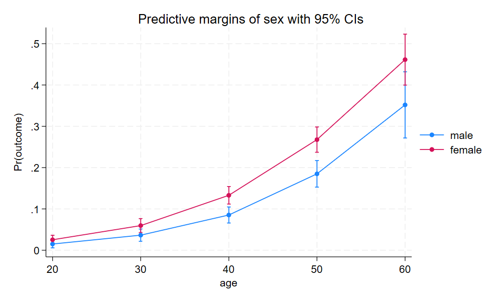
margins provides a lot of results, which can be difficult to understand. Therefore, we use marginsplot to plot these margins results.

There certainly seems to be some kind of interaction of sex and age.


marginsplot

graph export mymarginsplot.png, width(1000) replace

Running C:\Users\agrogan\Desktop\GitHub\newstuff\categorical\logistic-interacti
> ons-2\profile.do . 

Variables that uniquely identify margins: age sex

file mymarginsplot.png saved as PNG format

7 Rerun `margins`, `post`ing Results

We again employ the margins command, this time using the post option so that the results of the margins command are posted as an estimation result. This will allow us to employ the test command to statistically test different margins against each other.


margins sex, at(age = (20 30 40 50 60)) post

Running C:\Users\agrogan\Desktop\GitHub\newstuff\categorical\logistic-interacti
> ons-2\profile.do . 

Predictive margins                                       Number of obs = 3,000
Model VCE: OIM

Expression: Pr(outcome), predict()
1._at: age = 20
2._at: age = 30
3._at: age = 40
4._at: age = 50
5._at: age = 60

------------------------------------------------------------------------------
             |            Delta-method
             |     Margin   std. err.      z    P>|z|     [95% conf. interval]
-------------+----------------------------------------------------------------
     _at#sex |
     1#male  |   .0150645   .0047348     3.18   0.001     .0057846    .0243445
   1#female  |    .025333   .0055508     4.56   0.000     .0144536    .0362124
     2#male  |   .0364848   .0075444     4.84   0.000     .0216981    .0512714
   2#female  |   .0596255   .0086074     6.93   0.000     .0427552    .0764958
     3#male  |   .0852689   .0099016     8.61   0.000     .0658622    .1046757
   3#female  |   .1329912   .0108127    12.30   0.000     .1117987    .1541838
     4#male  |   .1849367   .0163684    11.30   0.000     .1528551    .2170182
   4#female  |    .267774   .0156218    17.14   0.000     .2371558    .2983921
     5#male  |   .3518378   .0408522     8.61   0.000      .271769    .4319066
   5#female  |   .4614446   .0314754    14.66   0.000     .3997539    .5231353
------------------------------------------------------------------------------

8 `margins` with `coeflegend`

We follow up by using the margins command with the coeflegend option to see the way in which Stata has labeled the different margins.


margins, coeflegend

Running C:\Users\agrogan\Desktop\GitHub\newstuff\categorical\logistic-interacti
> ons-2\profile.do . 

Predictive margins                                       Number of obs = 3,000
Model VCE: OIM

Expression: Pr(outcome), predict()
1._at: age = 20
2._at: age = 30
3._at: age = 40
4._at: age = 50
5._at: age = 60

------------------------------------------------------------------------------
             |     Margin   Legend
-------------+----------------------------------------------------------------
     _at#sex |
     1#male  |   .0150645  _b[1bn._at#0bn.sex]
   1#female  |    .025333  _b[1bn._at#1.sex]
     2#male  |   .0364848  _b[2._at#0bn.sex]
   2#female  |   .0596255  _b[2._at#1.sex]
     3#male  |   .0852689  _b[3._at#0bn.sex]
   3#female  |   .1329912  _b[3._at#1.sex]
     4#male  |   .1849367  _b[4._at#0bn.sex]
   4#female  |    .267774  _b[4._at#1.sex]
     5#male  |   .3518378  _b[5._at#0bn.sex]
   5#female  |   .4614446  _b[5._at#1.sex]
------------------------------------------------------------------------------

9 Testing Margins Against Each Other

Lastly, we test the margins at age 20 for men and women, and again at ages 50 and 60 for men and women.

We note that the original regression parameter for the interaction term was not statistically significant. Indeed, the margins at age 20 are not statistically significantly different by sex. However, at ages 50 & 60, there is a statistically significant difference by sex.


test _b[1bn._at#0bn.sex] = _b[1bn._at#1.sex] // male and female at age 20
    
test _b[4._at#0bn.sex] = _b[4._at#1.sex] // male and female at age 50

test _b[5._at#0bn.sex] =  _b[5._at#1.sex] // male and female at age 60

Running C:\Users\agrogan\Desktop\GitHub\newstuff\categorical\logistic-interacti
> ons-2\profile.do . 

 ( 1)  1bn._at#0bn.sex - 1bn._at#1.sex = 0

           chi2(  1) =    1.99
         Prob > chi2 =    0.1583


 ( 1)  4._at#0bn.sex - 4._at#1.sex = 0

           chi2(  1) =   13.03
         Prob > chi2 =    0.0003


 ( 1)  5._at#0bn.sex - 5._at#1.sex = 0

           chi2(  1) =    5.16
         Prob > chi2 =    0.0232

There is some suggestion that the difference of the differences is statistically significant. This statistical significance is only marginal [pun intended] at age 60, but truly statistically significant at age 50.


test _b[1bn._at#1.sex] - _b[1bn._at#0bn.sex] = _b[5._at#1.sex] - _b[5._at#0bn.sex] // test equivalence of the differences
    
test _b[1bn._at#1.sex] - _b[1bn._at#0bn.sex] = _b[4._at#1.sex] - _b[4._at#0bn.sex] // test equivalence of the differences

Running C:\Users\agrogan\Desktop\GitHub\newstuff\categorical\logistic-interacti
> ons-2\profile.do . 

 ( 1)  - 1bn._at#0bn.sex + 1bn._at#1.sex + 5._at#0bn.sex - 5._at#1.sex = 0

           chi2(  1) =    3.62
         Prob > chi2 =    0.0572


 ( 1)  - 1bn._at#0bn.sex + 1bn._at#1.sex + 4._at#0bn.sex - 4._at#1.sex = 0

           chi2(  1) =    9.77
         Prob > chi2 =    0.0018

References

Ai, Chunrong, and Edward C. Norton. 2003. “Interaction Terms in Logit and Probit Models.” Economics Letters. https://doi.org/10.1016/S0165-1765(03)00032-6.

Karaca-Mandic, Pinar, Edward C. Norton, and Bryan Dowd. 2012. “Interaction Terms in Nonlinear Models.” Health Services Research. https://doi.org/10.1111/j.1475-6773.2011.01314.x.

1 Background

2 Get The Data

3 Describe The Data

4 Estimate Logistic Regression

5 Margins

6 Plotting Margins

7 Rerun margins, posting Results

8 margins with coeflegend

9 Testing Margins Against Each Other

References

7 Rerun `margins`, `post`ing Results

8 `margins` with `coeflegend`