Interactions in Logistic Regression

New Version

Author

Andy Grogan-Kaylor

Published

April 25, 2024

1 Background

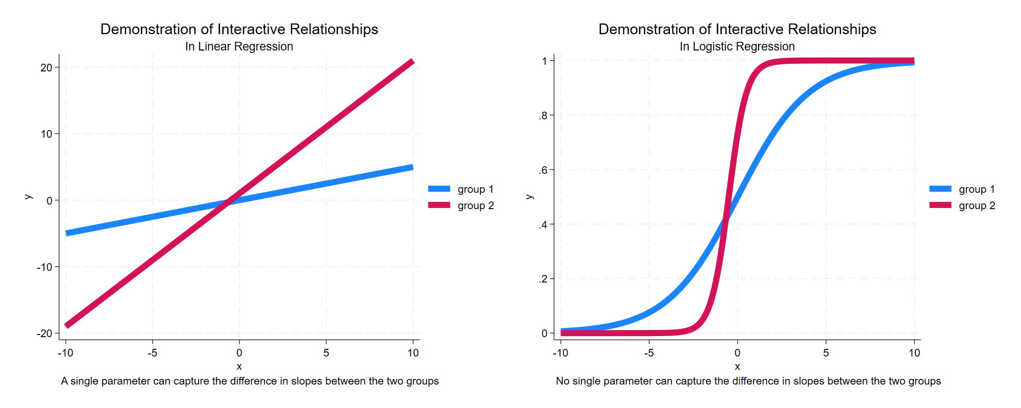
The purpose of this tutorial is to illustrate the idea that in logistic regression, the \(\beta\) parameter for an interaction term may not accurately characterize the underlying interactive relationships.

This idea may be easier to describe if we recall the formula for a logistic regression:

\[\ln\left(\frac{P(y)}{1 - P(y)}\right) = \beta_0 + \beta_1 x_1 + \beta_2 x_2 + \beta_3 x_1 \times x_2 \tag{1}\]

Warning

In the above formula, the sign, and statistical significance, of \(\beta_3\) may not accurately characterize the underlying relationship.

Demonstration of Interactive Relationships

Key Idea

In a linear model, a single parameter can capture the difference in slopes between the two groups. In a non-linear model, no single parameter can capture the difference in slopes between the two groups.

Some Calculus (Not Essential To The Discussion)

Imagine a linear model:

\[y = \beta_0 + \beta_1 x_1 + \beta_2 x_2 + \beta_3 x_1 \times x_2 + e_i\]

Here (following Ai and Norton (2003)):

\[\frac{\partial y}{\partial x_1 \partial x_2} = \beta_3\]

We use \(\text{logit}\) to describe:

\[\ln\left(\frac{P(y)}{1 - P(y)}\right)\]

In the logistic model, the quantity:

\[\frac{\partial \text{logit} (y)}{\partial x_1 \partial x_2}\]

does not have such a straightforward solution, and–importantly for this discussion–is not simply equal to \(\beta_3\).

2 Get The Data

We start by obtaining simulated data from StataCorp.


clear all

graph close _all

use http://www.stata-press.com/data/r15/margex, clear

(Artificial data for margins)

3 Describe The Data

The variables are as follows:


describe

Running C:\Users\agrogan\Desktop\GitHub\newstuff\categorical\logistic-interacti
> ons-3\profile.do . 

Contains data from http://www.stata-press.com/data/r15/margex.dta
 Observations:         3,000                  Artificial data for margins
    Variables:            11                  27 Nov 2016 14:27
-------------------------------------------------------------------------------
Variable      Storage   Display    Value
    name         type    format    label      Variable label
-------------------------------------------------------------------------------
y               float   %6.1f                 
outcome         byte    %2.0f                 
sex             byte    %6.0f      sexlbl     
group           byte    %2.0f                 
age             float   %3.0f                 
distance        float   %6.2f                 
ycn             float   %6.1f                 
yc              float   %6.1f                 
treatment       byte    %2.0f                 
agegroup        byte    %8.0g      agelab     
arm             byte    %8.0g                 
-------------------------------------------------------------------------------
Sorted by: group

4 Estimate Logistic Regression

We then run a logistic regression model in which outcome is the dependent variable. age and group are the independent variables. We estimate an interaction of group and age.

We note that the regression coefficient for the interaction terms are not statistically significant.


logit outcome c.age##i.group

Running C:\Users\agrogan\Desktop\GitHub\newstuff\categorical\logistic-interacti
> ons-3\profile.do . 

Iteration 0:  Log likelihood = -1366.0718  
Iteration 1:  Log likelihood = -1125.2149  
Iteration 2:  Log likelihood =  -1077.539  
Iteration 3:  Log likelihood = -1074.8422  
Iteration 4:  Log likelihood = -1074.7864  
Iteration 5:  Log likelihood = -1074.7863  

Logistic regression                                     Number of obs =  3,000
                                                        LR chi2(5)    = 582.57
                                                        Prob > chi2   = 0.0000
Log likelihood = -1074.7863                             Pseudo R2     = 0.2132

------------------------------------------------------------------------------
     outcome | Coefficient  Std. err.      z    P>|z|     [95% conf. interval]
-------------+----------------------------------------------------------------
         age |    .091183   .0084697    10.77   0.000     .0745827    .1077834
             |
       group |
          2  |  -.8272665   .6648279    -1.24   0.213    -2.130305    .4757722
          3  |  -1.085445   1.044802    -1.04   0.299    -3.133219    .9623292
             |
 group#c.age |
          2  |   .0013522   .0139747     0.10   0.923    -.0260378    .0287421
          3  |  -.0164596   .0259182    -0.64   0.525    -.0672584    .0343392
             |
       _cons |  -5.184398   .4274964   -12.13   0.000    -6.022275    -4.34652
------------------------------------------------------------------------------

5 Margins

We use the margins command to estimate predicted probabilities at different values of group and age.


margins group, at(age = (20 30 40 50 60))

Running C:\Users\agrogan\Desktop\GitHub\newstuff\categorical\logistic-interacti
> ons-3\profile.do . 

Adjusted predictions                                     Number of obs = 3,000
Model VCE: OIM

Expression: Pr(outcome), predict()
1._at: age = 20
2._at: age = 30
3._at: age = 40
4._at: age = 50
5._at: age = 60

------------------------------------------------------------------------------
             |            Delta-method
             |     Margin   std. err.      z    P>|z|     [95% conf. interval]
-------------+----------------------------------------------------------------
   _at#group |
        1 1  |   .0335453   .0084761     3.96   0.000     .0169325    .0501582
        1 2  |   .0153532   .0044572     3.44   0.001     .0066173    .0240891
        1 3  |   .0083644   .0041378     2.02   0.043     .0002545    .0164742
        2 1  |   .0795185   .0132311     6.01   0.000     .0535861     .105451
        2 2  |   .0378475   .0070835     5.34   0.000      .023964    .0517309
        2 3  |   .0174959   .0054051     3.24   0.001     .0069021    .0280896
        3 1  |   .1769607   .0155126    11.41   0.000     .1465565    .2073649
        3 2  |   .0902771   .0095282     9.47   0.000     .0716022     .108952
        3 3  |   .0362321   .0091647     3.95   0.000     .0182697    .0541945
        4 1  |   .3485893   .0149941    23.25   0.000     .3192014    .3779772
        4 2  |   .2002224   .0188064    10.65   0.000     .1633625    .2370823
        4 3  |   .0735312   .0271556     2.71   0.007     .0203072    .1267553
        5 1  |   .5711598   .0265203    21.54   0.000     .5191809    .6231386
        5 2  |   .3870919   .0467552     8.28   0.000     .2954535    .4787304
        5 3  |   .1435103   .0746567     1.92   0.055    -.0028141    .2898347
------------------------------------------------------------------------------

6 Plotting Margins

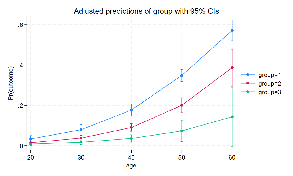
margins provides a lot of results, which can be difficult to understand. Therefore, we use marginsplot to plot these margins results.

There certainly seems to be some kind of interaction of group and age.


marginsplot

graph export mymarginsplot.png, width(1000) replace

Running C:\Users\agrogan\Desktop\GitHub\newstuff\categorical\logistic-interacti
> ons-3\profile.do . 

Variables that uniquely identify margins: age group

file mymarginsplot.png saved as PNG format

7 Rerun `margins`, `post`ing Results

We again employ the margins command, this time using the post option so that the results of the margins command are posted as an estimation result. This will allow us to employ the test command to statistically test different margins against each other.


margins group, at(age = (20 30 40 50 60)) post

Running C:\Users\agrogan\Desktop\GitHub\newstuff\categorical\logistic-interacti
> ons-3\profile.do . 

Adjusted predictions                                     Number of obs = 3,000
Model VCE: OIM

Expression: Pr(outcome), predict()
1._at: age = 20
2._at: age = 30
3._at: age = 40
4._at: age = 50
5._at: age = 60

------------------------------------------------------------------------------
             |            Delta-method
             |     Margin   std. err.      z    P>|z|     [95% conf. interval]
-------------+----------------------------------------------------------------
   _at#group |
        1 1  |   .0335453   .0084761     3.96   0.000     .0169325    .0501582
        1 2  |   .0153532   .0044572     3.44   0.001     .0066173    .0240891
        1 3  |   .0083644   .0041378     2.02   0.043     .0002545    .0164742
        2 1  |   .0795185   .0132311     6.01   0.000     .0535861     .105451
        2 2  |   .0378475   .0070835     5.34   0.000      .023964    .0517309
        2 3  |   .0174959   .0054051     3.24   0.001     .0069021    .0280896
        3 1  |   .1769607   .0155126    11.41   0.000     .1465565    .2073649
        3 2  |   .0902771   .0095282     9.47   0.000     .0716022     .108952
        3 3  |   .0362321   .0091647     3.95   0.000     .0182697    .0541945
        4 1  |   .3485893   .0149941    23.25   0.000     .3192014    .3779772
        4 2  |   .2002224   .0188064    10.65   0.000     .1633625    .2370823
        4 3  |   .0735312   .0271556     2.71   0.007     .0203072    .1267553
        5 1  |   .5711598   .0265203    21.54   0.000     .5191809    .6231386
        5 2  |   .3870919   .0467552     8.28   0.000     .2954535    .4787304
        5 3  |   .1435103   .0746567     1.92   0.055    -.0028141    .2898347
------------------------------------------------------------------------------

8 `margins` with `coeflegend`

We follow up by using the margins command with the coeflegend option to see the way in which Stata has labeled the different margins.


margins, coeflegend

Running C:\Users\agrogan\Desktop\GitHub\newstuff\categorical\logistic-interacti
> ons-3\profile.do . 

Adjusted predictions                                     Number of obs = 3,000
Model VCE: OIM

Expression: Pr(outcome), predict()
1._at: age = 20
2._at: age = 30
3._at: age = 40
4._at: age = 50
5._at: age = 60

------------------------------------------------------------------------------
             |     Margin   Legend
-------------+----------------------------------------------------------------
   _at#group |
        1 1  |   .0335453  _b[1bn._at#1bn.group]
        1 2  |   .0153532  _b[1bn._at#2.group]
        1 3  |   .0083644  _b[1bn._at#3.group]
        2 1  |   .0795185  _b[2._at#1bn.group]
        2 2  |   .0378475  _b[2._at#2.group]
        2 3  |   .0174959  _b[2._at#3.group]
        3 1  |   .1769607  _b[3._at#1bn.group]
        3 2  |   .0902771  _b[3._at#2.group]
        3 3  |   .0362321  _b[3._at#3.group]
        4 1  |   .3485893  _b[4._at#1bn.group]
        4 2  |   .2002224  _b[4._at#2.group]
        4 3  |   .0735312  _b[4._at#3.group]
        5 1  |   .5711598  _b[5._at#1bn.group]
        5 2  |   .3870919  _b[5._at#2.group]
        5 3  |   .1435103  _b[5._at#3.group]
------------------------------------------------------------------------------

9 Testing Margins Against Each Other

Lastly, we test the margins at age 20 across some of the groups, and again at ages 50 and 60 for some of the groups.

We note that the original regression parameter for the interaction term was not statistically significant. Indeed, the margins at age 20 are not statistically significantly different by group (1 vs. 2), though they are close to being significantly different. However, at ages 50 & 60, there is a statistically significant difference by group (1 vs. 2).


test _b[1bn._at#1bn.group] = _b[1bn._at#2.group] // groups 1 & 2 at age 20
    
test _b[4._at#1bn.group] = _b[4._at#2.group] // groups 1 & 2 at age 50

test _b[5._at#1bn.group] =  _b[5._at#2.group] // groups 1 & 2 at age 60

Running C:\Users\agrogan\Desktop\GitHub\newstuff\categorical\logistic-interacti
> ons-3\profile.do . 

 ( 1)  1bn._at#1bn.group - 1bn._at#2.group = 0

           chi2(  1) =    3.61
         Prob > chi2 =    0.0575


 ( 1)  4._at#1bn.group - 4._at#2.group = 0

           chi2(  1) =   38.05
         Prob > chi2 =    0.0000


 ( 1)  5._at#1bn.group - 5._at#2.group = 0

           chi2(  1) =   11.73
         Prob > chi2 =    0.0006

References

Ai, Chunrong, and Edward C. Norton. 2003. “Interaction Terms in Logit and Probit Models.” Economics Letters. https://doi.org/10.1016/S0165-1765(03)00032-6.

Karaca-Mandic, Pinar, Edward C. Norton, and Bryan Dowd. 2012. “Interaction Terms in Nonlinear Models.” Health Services Research. https://doi.org/10.1111/j.1475-6773.2011.01314.x.

1 Background

2 Get The Data

3 Describe The Data

4 Estimate Logistic Regression

5 Margins

6 Plotting Margins

7 Rerun margins, posting Results

8 margins with coeflegend

9 Testing Margins Against Each Other

References

7 Rerun `margins`, `post`ing Results

8 `margins` with `coeflegend`