Background

I shared some of my handouts and slides on logistic regression with Madhur Singh, who was a visiting student at the University of Michigan School of Social Work. He wrote back with the following response, which I thought was exceptionally thoughtful.

Madhur Writes:

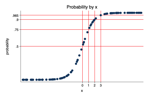
“To get a better grip of the distinction between odds and probability, I was trying to ‘visualize’ it mathematically, and very interestingly, if we assume that the odds of an event, y, at x = 0 is 1 (i.e., p = 0.5) and OR = 3 (i.e., a 200% increase in the odds for every unit increase in x), (NB: Here, p is the probability of the event occurring; NOT the ‘p-value’ from the regression)”

“Then: A unit increase in x from 0 –> 1 will increase the odds to 3. This is equivalent to p = 0.75 (at x = 1), which is a 50% increase in the predicted probability (0.5 + 0.25).”

“For the next unit increase in x form 1 –> 2, the odds for y increase to 9, which gives a predicted probability of 0.9 at x = 1, or a 20% increase (a ‘slower’ change compared to the 50% increase with the first unit change in x).”

“And for the next unit increase in x from 2 –> 3, the odds for y increase to (whopping) 27, equivalent to a predicted probability of 0.965 at x = 2, which in fact is a much smaller 7.2% increase in the predicted probability.”

Below, I try to visualize Madhur’s ideas.

. clear all // clear the workspace

. set obs 100 // 100 simulated observations
number of observations (_N) was 0, now 100

. generate x = runiform(-10,10) // randomly distributed x

. generate p = exp(1.0986123 *x)/(1 + exp(1.0986123 *x)) // p with odds ratio of 3 CF ln(3)

. twoway scatter p x, ///
> title("Probability by x") ytitle("probability") ///
> xline(0 1 2 3, lcolor("red")) yline(.5 .75 .9 .965, lcolor("red")) ///
> xlabel(0 1 2 3) ylabel(.5 .75 .9 .965) ///
> scheme(michigan) // graph

. graph export myscatter.png, width(500) replace
(file myscatter.png written in PNG format)

Madhur goes on to write:

“So, if y were a desirable outcome, and one were to design an intervention to increase x as a way to effect an increase in the likelihood of y in the population, then to ‘anecdotally’ examine the effectiveness of the intervention, one might expect the most immediate ‘real-world’ change among those whose baseline levels of x are somewhere close to 0.”

“By extension, among those with the baseline levels of x way below 0, it’d be helpful to be patient and persistent with the efforts to raise the levels of x before one sees an appreciable change in y (even though, empirically, the change in odds will be mathematically proportional in both groups).”