predict and margins: A Substantive Example1 Mar 2021 08:09:03
Odds ratios, or coefficients showing the association of the independent variables with the log odds, represent the most immediate output of a logistic regression. However, for a variety of reasons, it may make sense to not only report odds ratios, but also to investigate predicted probabilities.
The data are an extract of the National Survey of Children’s Health, 2018. The data contain information on children’s current depression status, their exposure to various Adverse Childhood Experiences (ACEs) and their sex and race.
. clear all
. cd "/Users/agrogan/Desktop/newstuff/categorical/predict-and-margins-substantive-example"
/Users/agrogan/Desktop/newstuff/categorical/predict-and-margins-substantive-example
. use "NSCH_ACES.dta", clear
. describe depress ace1R ace3R ace4R ace5R ace6R ace7R ace8R ace9R

              storage   display    value
variable name   type    format     label      variable label
──────────────────────────────────────────────────────────────────────────────────────────────────────
depress         byte    %9.0g                 RECODE of k2q32b (Depression Currently)
ace1R           byte    %9.0g                 RECODE of ace1 (Hard to Cover Basics Like Food or
                                                Housing)
ace3R           byte    %9.0g                 RECODE of ace3 (Child Experienced - Parent or Guardian
                                                Divorced)
ace4R           byte    %9.0g                 RECODE of ace4 (Child Experienced - Parent or Guardian
                                                Died)
ace5R           byte    %9.0g                 RECODE of ace5 (Child Experienced - Parent or Guardian
                                                Time in Jail)
ace6R           byte    %9.0g                 RECODE of ace6 (Child Experienced - Adults Slap, Hit,
                                                Kick, Punch Others)
ace7R           byte    %9.0g                 RECODE of ace7 (Child Experienced - Victim of Violence)
ace8R           byte    %9.0g                 RECODE of ace8 (Child Experienced - Lived with Mentally
                                                Ill)
ace9R           byte    %9.0g                 RECODE of ace9 (Child Experienced - Lived with Person
                                                with Alcohol/Drug Problem)
We estimate a logistic regression using ,or to ask for odds ratios.
. logit depress ace1R ace3R ace4R ace5R ace6R ace7R ace8R ace9R i.sc_race_r i.sc_sex, or

Iteration 0:   log likelihood = -760.76202
Iteration 1:   log likelihood = -739.43605
Iteration 2:   log likelihood =   -739.012
Iteration 3:   log likelihood = -739.01149
Iteration 4:   log likelihood = -739.01149

Logistic regression                             Number of obs     =      1,442
                                                LR chi2(15)       =      43.50
                                                Prob > chi2       =     0.0001
Log likelihood = -739.01149                     Pseudo R2         =     0.0286

────────────────────────────────────┬────────────────────────────────────────────────────────────────
                            depress │ Odds Ratio   Std. Err.      z    P>|z|     [95% Conf. Interval]
────────────────────────────────────┼────────────────────────────────────────────────────────────────
                              ace1R │   1.275539    .177745     1.75   0.081      .970688     1.67613
                              ace3R │   .8328396   .1225773    -1.24   0.214     .6241393    1.111325
                              ace4R │    1.03589   .2559531     0.14   0.887     .6382551    1.681253
                              ace5R │   1.238661   .2620121     1.01   0.312     .8182749     1.87502
                              ace6R │   1.242079    .284433     0.95   0.344     .7929142    1.945684
                              ace7R │   1.438336   .3249996     1.61   0.108     .9236915     2.23972
                              ace8R │   1.931751   .3179664     4.00   0.000     1.399082    2.667221
                              ace9R │   .6476801   .1088199    -2.59   0.010     .4659572    .9002747
                                    │
                          sc_race_r │
   Black or African American alone  │   1.150371   .3258065     0.49   0.621     .6603312    2.004075
American Indian or Alaska Native..  │   .7002442   .4236335    -0.59   0.556      .213939    2.291971
                       Asian alone  │   1.222781   .5325791     0.46   0.644     .5207269    2.871358
Native Hawaiian and Other Pacifi..  │   .2318806   .3550441    -0.95   0.340     .0115331    4.662103
             Some Other Race alone  │   .7923493   .3360807    -0.55   0.583     .3450431    1.819533
                 Two or More Races  │   .7852821   .1983556    -0.96   0.339     .4786515    1.288345
                                    │
                             sc_sex │
                            Female  │    1.36572   .1769313     2.41   0.016     1.059466    1.760501
                              _cons │   2.357814   .3247614     6.23   0.000     1.799975    3.088536
────────────────────────────────────┴────────────────────────────────────────────────────────────────
Note: _cons estimates baseline odds.
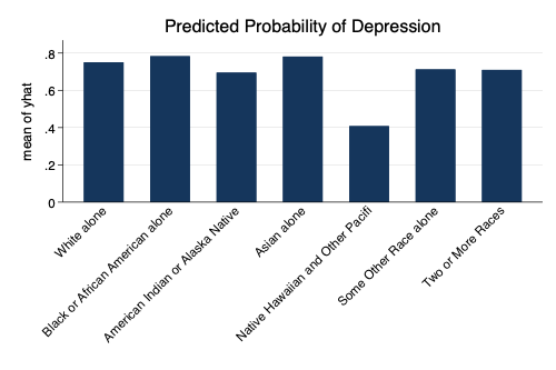
Predicted probabilities are each participant’s individual predicted probability of experiencing depression based upon the independent variables included in the model. We often denote such predicted probabilities with \(\hat{y}\)
. predict yhat
(option pr assumed; Pr(depress))
(1,558 missing values generated)
yhat is a variable in the data, just like any other variable, and we can tabulate and graph it.
. tabulate sc_race_r, summarize(yhat)

    Race of │
   Selected │
     Child, │       Summary of Pr(depress)
   Detailed │        Mean   Std. Dev.       Freq.
────────────┼────────────────────────────────────
  White alo │   .75045109   .05197594      22,445
  Black or  │   .78322165   .04940146       1,881
  American  │   .69508786   .07204945         235
  Asian alo │   .78128584   .03714901       1,377
  Native Ha │   .40799774   .06911794          73
  Some Othe │   .71235484   .05558899         763
  Two or Mo │   .70971281   .06233783       2,198
────────────┼────────────────────────────────────
      Total │   .74863835   .05781597      28,972
. graph bar yhat, ///
> over(sc_race_r, label(angle(forty_five))) ///
> title("Predicted Probability of Depression") ///
> scheme(michigan)
. graph export mybar.png, width(500) replace
(file /Users/agrogan/Desktop/newstuff/categorical/predict-and-margins-substantive-example/mybar.png wr
> itten in PNG format)
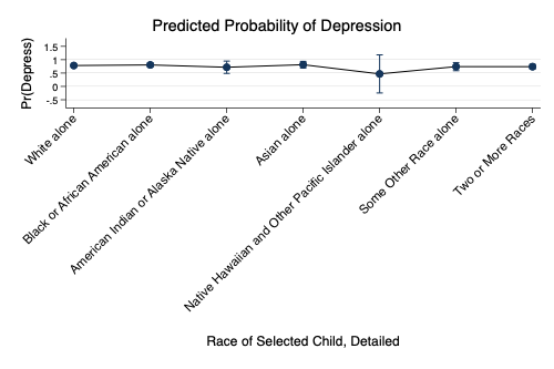
In their simplest form, predictive margins are average predicted probabilities were everyone in the sample were treated as if they were of a particular race.
. margins sc_race_r // predictive margins

Predictive margins                              Number of obs     =      1,442
Model VCE    : OIM

Expression   : Pr(depress), predict()

────────────────────────────────────┬────────────────────────────────────────────────────────────────
                                    │            Delta-method
                                    │     Margin   Std. Err.      z    P>|z|     [95% Conf. Interval]
────────────────────────────────────┼────────────────────────────────────────────────────────────────
                          sc_race_r │
                       White alone  │   .7819423    .011883    65.80   0.000      .758652    .8052326
   Black or African American alone  │   .8043012   .0419853    19.16   0.000     .7220115    .8865909
American Indian or Alaska Native..  │   .7173792   .1176945     6.10   0.000     .4867023    .9480561
                       Asian alone  │   .8135006   .0635869    12.79   0.000     .6888727    .9381286
Native Hawaiian and Other Pacifi..  │   .4675318   .3641302     1.28   0.199    -.2461503    1.181214
             Some Other Race alone  │   .7409869   .0777287     9.53   0.000     .5886414    .8933323
                 Two or More Races  │   .7393176   .0451682    16.37   0.000     .6507896    .8278456
────────────────────────────────────┴────────────────────────────────────────────────────────────────
We could also evaluate
marginsholding other variables at their mean values using theatmeansoption. You can also read about obtainingmarginsfor various combinations of the independent variables by typinghelp marginsat the Stata prompt.
The essential graphing command is marginsplot, which will usually produce a perfectly useable graph. The other graphing options are added for clarification and aesthetic purposes.
. marginsplot, ///
> title("Predicted Probability of Depression") ///
> ylabel(, labsize(small) angle(horizontal)) ///
> xlabel(, angle(forty_five)) ///
> scheme(michigan)

  Variables that uniquely identify margins: sc_race_r
. graph export mymargins.png, width(500) replace
(file /Users/agrogan/Desktop/newstuff/categorical/predict-and-margins-substantive-example/mymargins.pn
> g written in PNG format)