Introduction
“Survival analysis is a key technique in data-driven decision-making,
which is now central to public interest because of COVID-19. Applying
the correct technique for the specific question at hand is crucial for
credible public health inferences. If you are interested in assessing
how a risk factor or a potential treatment affects the progression of a
disease—such as how long a patient takes to recover—then survival
analysis techniques come into play. Survival analysis deeply respects
the ultimate source of its data, often the disease experience or even
the life and death of human patients. It seeks to exploit every last
drop of information that this experience can render for saving lives—in
particular, not only whether patients survived, but how long, and why.
And it strives to do so with minimal assumptions, so that the data are
truly driving the decision.”
—SAS Corporation
Setup of Data
. stset // show st setup of data
-> stset studytime, failure(died)

Survival-time data settings

         Failure event: died!=0 & died<.
Observed time interval: (0, studytime]
     Exit on or before: failure

──────────────────────────────────────────────────────────────────────────
         48  total observations
          0  exclusions
──────────────────────────────────────────────────────────────────────────
         48  observations remaining, representing
         31  failures in single-record/single-failure data
        744  total analysis time at risk and under observation
                                                At risk from t =         0
                                     Earliest observed entry t =         0
                                          Last observed exit t =        39
. describe // show variables in data

Contains data from https://www.stata-press.com/data/r18/drugtr.dta
 Observations:            48                  Patient survival in drug trial
    Variables:             8                  3 Mar 2022 02:12
───────────────────────────────────────────────────────────────────────────────────────
Variable      Storage   Display    Value
    name         type    format    label      Variable label
───────────────────────────────────────────────────────────────────────────────────────
studytime       byte    %8.0g                 Months to death or end of exp.
died            byte    %8.0g                 1 if patient died
drug            byte    %8.0g                 Drug type (0=placebo)
age             byte    %8.0g                 Patient's age at start of exp.
_st             byte    %8.0g                 1 if record is to be used; 0 otherwise
_d              byte    %8.0g                 1 if failure; 0 if censored
_t              byte    %10.0g                Analysis time when record ends
_t0             byte    %10.0g                Analysis time when record begins
───────────────────────────────────────────────────────────────────────────────────────
Sorted by:
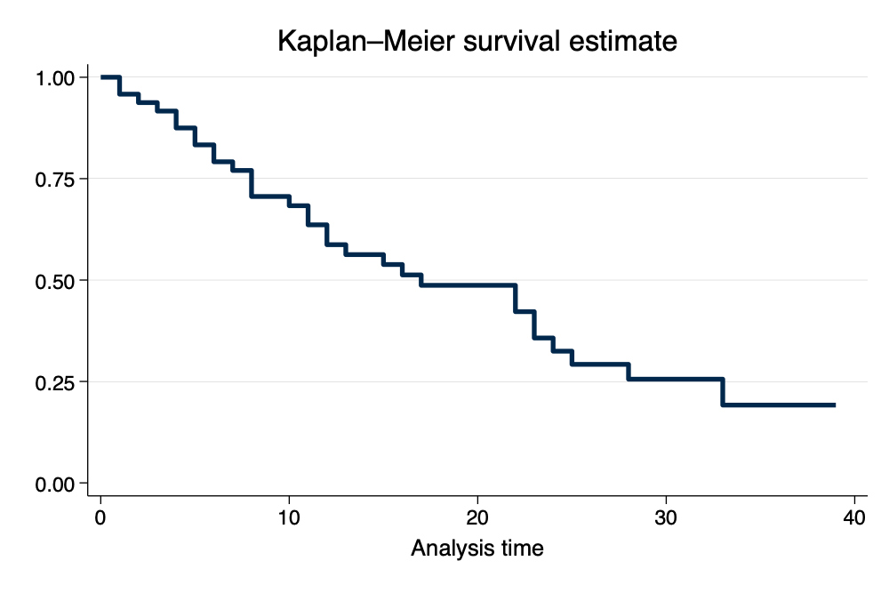
Kaplan-Meier Survivor Function (per Gabriela Ortiz, Stata)
\[ S(t)=Pr(T>t) \]
. sts graph, scheme(michigan) // Kaplan-Meier Survivor Function

        Failure _d: died
  Analysis time _t: studytime
. graph export survival0.png, width(1000) replace
file
    /Users/agrogan/Desktop/GitHub/newstuff/categorical/survival-analysis-and-event-hi
    > story/survival0.png saved as PNG format

Kaplan-Meier Survivor Function
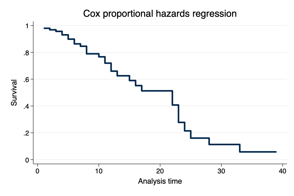
Graph Survival Curves
. stcurve, survival scheme(michigan) // survival curve
note: function evaluated at overall means of covariates.
. graph export survival1.png, width(1000) replace
file
    /Users/agrogan/Desktop/GitHub/newstuff/categorical/survival-analysis-and-event-hi
    > story/survival1.png saved as PNG format

Survival Curve
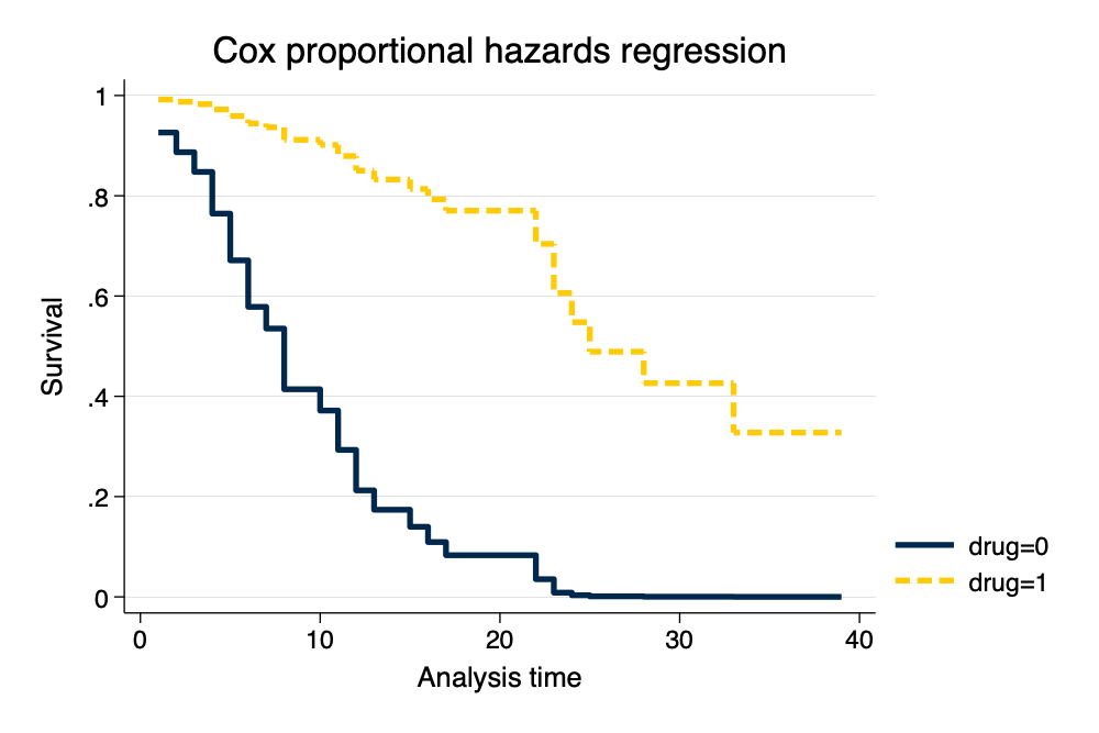
. stcurve, survival at1(drug=0) at2(drug=1) scheme(michigan) // survival curve by group
note: function evaluated at specified values of selected covariates and overall means
      of other covariates (if any).
. graph export survival2.png, width(1000) replace
file
    /Users/agrogan/Desktop/GitHub/newstuff/categorical/survival-analysis-and-event-hi
    > story/survival2.png saved as PNG format

Survival Curve by Drug Group
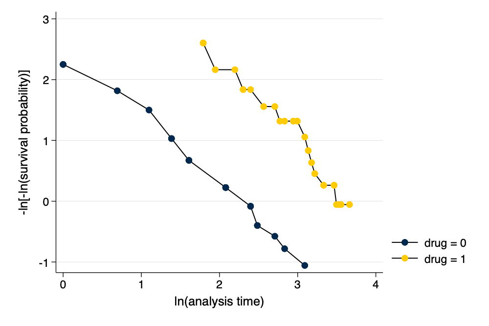
Proportional Hazards Assumption
. estat phtest // formal test of PH assumption

Test of proportional-hazards assumption

Time function: Analysis time
─────────────┬──────────────────────────────────
             │     chi2       df       Prob>chi2
─────────────┼──────────────────────────────────
 Global test │     0.43        2          0.8064
─────────────┴──────────────────────────────────
. stphplot, by(drug) scheme(michigan) // graphical test of PH assumption

        Failure _d: died
  Analysis time _t: studytime
. graph export ph.png, width(1000) replace
file
    /Users/agrogan/Desktop/GitHub/newstuff/categorical/survival-analysis-and-event-hi
    > story/ph.png saved as PNG format

Graphical Assessment of Proportional Hazards
Assumptions
References
Johnson, L. L., & Shih, J. H. (2007). CHAPTER 20 - An
Introduction to Survival Analysis (J. I. Gallin & F. P. Ognibene,
eds.).
https://doi.org/https://doi.org/10.1016/B978-012369440-9/50024-4
Ragnar Frisch Centre for Economic Research (2020). Event History
Analysis, Survival Analysis, Duration Analysis ,Transition Data
Analysis, Hazard Rate Analysis. Oslo, Norway.
