5 Nov 2023
This example uses data on the ages of death of Roman Emperors. Sources for this data are unclear, but it appears that the original source is http://www.roman-emperors.org/ via https://github.com/rfordatascience/tidytuesday/tree/master/data/2019/2019-08-13.
. clear all
. import delimited "https://raw.githubusercontent.com/agrogan1/newstuff/master/categori
> cal/survival-analysis-and-event-history/emperors/emperors.csv"
(encoding automatically selected: ISO-8859-1)
(16 vars, 68 obs)
Remember that Stata works with dates by converting them to the number of days since January 1, 1960.
. * we can't use the date() function
. * because it does not work
. * with dates prior to 100AD
. * generate birthdate = date(birth, "YMD")
. * generate deathdate = date(death, "YMD")
. generate birthyear = real(substr(birth, 1, 4)) // convert first 4 characters to real
> number
(5 missing values generated)
. generate deathyear = real(substr(death, 1, 4)) // convert first 4 characters to real
> number
. * browse name name_full birth birthyear death deathyear
. generate age = deathyear - birthyear
(5 missing values generated)
. * need to recalculate age for those born in BCE
. encode cause, generate(causeNUMERIC) // numeric version of cause of death
. codebook causeNUMERIC if age != . // show values of causeNUMERIC for non missing ages

───────────────────────────────────────────────────────────────────────────────────────
causeNUMERIC                                                                (unlabeled)
───────────────────────────────────────────────────────────────────────────────────────

                  Type: Numeric (long)
                 Label: causeNUMERIC

                 Range: [1,7]                         Units: 1
         Unique values: 7                         Missing .: 0/63

            Tabulation: Freq.   Numeric  Label
                           23         1  Assassination
                            1         2  Captivity
                            4         3  Died in Battle
                            8         4  Execution
                           21         5  Natural Causes
                            5         6  Suicide
                            1         7  Unknown
. encode rise, generate(riseNUMERIC) // numeric version of cause of death
. codebook riseNUMERIC // show values of riseNUMERIC

───────────────────────────────────────────────────────────────────────────────────────
riseNUMERIC                                                                 (unlabeled)
───────────────────────────────────────────────────────────────────────────────────────

                  Type: Numeric (long)
                 Label: riseNUMERIC

                 Range: [1,8]                         Units: 1
         Unique values: 8                         Missing .: 0/68

            Tabulation: Freq.   Numeric  Label
                            7         1  Appointment by Army
                            4         2  Appointment by Emperor
                            3         3  Appointment by Praetorian Guard
                            7         4  Appointment by Senate
                           35         5  Birthright
                            1         6  Election
                            1         7  Purchase
                           10         8  Seized Power
stset The Data
We need to stset the data so that Stata knows that this
is survival data with special characteristics relevant to survival
analysis. For those of you have used other commands that attach special
characteristics to the data, this is similar to using
svyset for complex survey data, xtset for
panel data, or even to the mi suite of commands for
multiple imputation.
The most commonly used syntax is something like
stset timevar, failure(failvar) id(id) 1
There are many ways to specify
failvar, we outline the most straightforward. Consult Stata help for your exact situation.
. stset age // stset the data

Survival-time data settings

         Failure event: (assumed to fail at time=age)
Observed time interval: (0, age]
     Exit on or before: failure

──────────────────────────────────────────────────────────────────────────
         68  total observations
          5  event time missing (age>=.)                    PROBABLE ERROR
          2  observations end on or before enter()
──────────────────────────────────────────────────────────────────────────
         61  observations remaining, representing
         61  failures in single-record/single-failure data
      2,984  total analysis time at risk and under observation
                                                At risk from t =         0
                                     Earliest observed entry t =         0
                                          Last observed exit t =        79
\[S(t)=Pr(T>t)\]
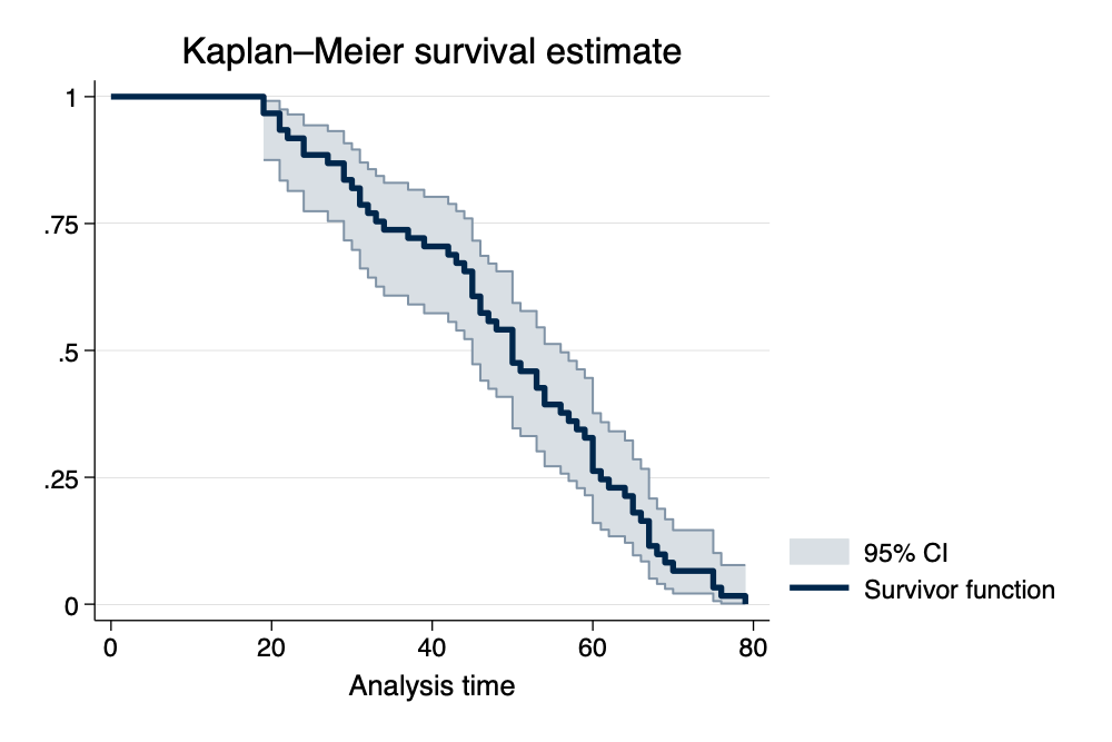
. sts graph, scheme(michigan) ci // survival graph with CI's

        Failure _d: 1 (meaning all fail)
  Analysis time _t: age
. graph export mysurvival0.png, width(1000) replace
file
    /Users/agrogan/Desktop/GitHub/newstuff/categorical/survival-analysis-and-event-hi
    > story/emperors/mysurvival0.png saved as PNG format
. sts graph, by(causeNUMERIC) scheme(michigan) // survival curve by cause of death

        Failure _d: 1 (meaning all fail)
  Analysis time _t: age
. graph export mysurvival1.png, width(1000) replace
file
    /Users/agrogan/Desktop/GitHub/newstuff/categorical/survival-analysis-and-event-hi
    > story/emperors/mysurvival1.png saved as PNG format
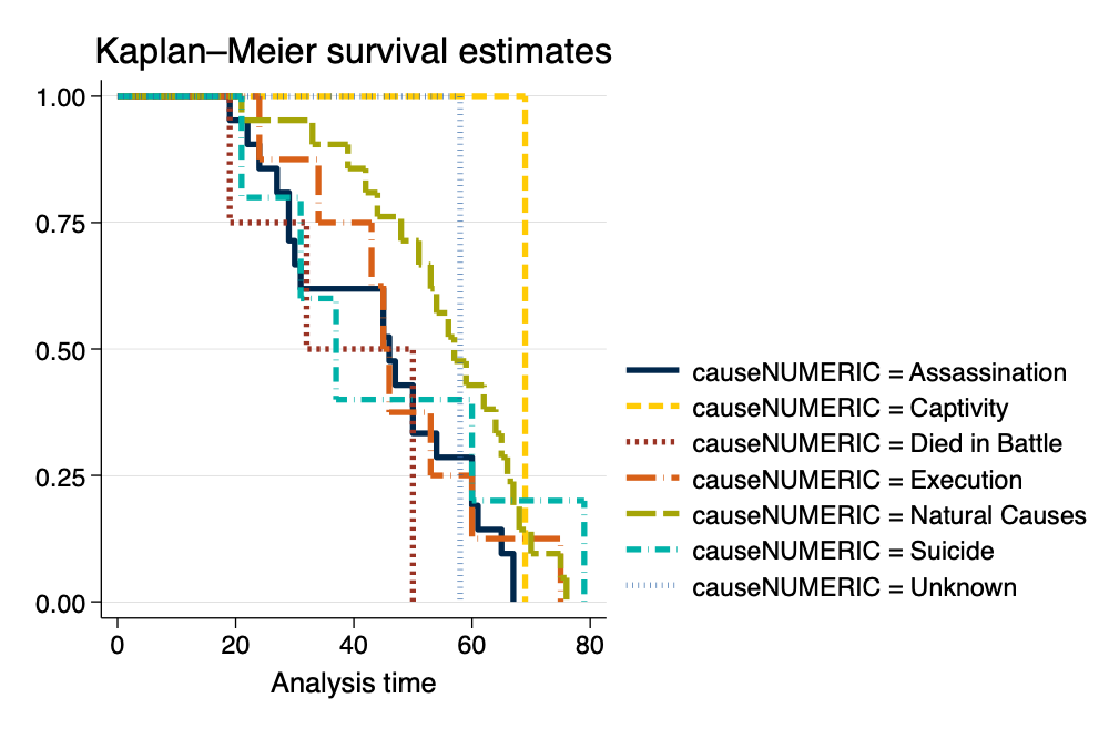
As an opportunity to take a closer look at the graph, we take a look at cause of death by age for those who died in battle.
. tabulate age causeNUMERIC if causeNUMERIC == 3

           │ causeNUMER
           │     IC
       age │ Died in B │     Total
───────────┼───────────┼──────────
        19 │         1 │         1
        32 │         1 │         1
        50 │         2 │         2
───────────┼───────────┼──────────
     Total │         4 │         4
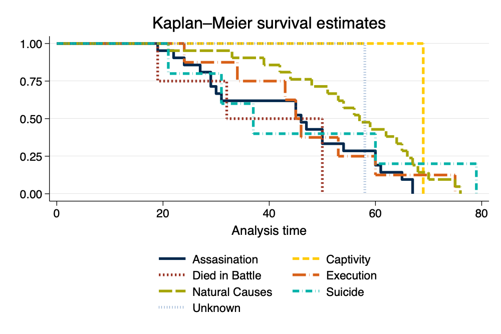
We can then work to make the legend more informative.
. sts graph, by(causeNUMERIC) scheme(michigan) ///
> legend(pos(6) col(2) order(1 "Assasination" 2 "Captivity" 3 "Died in Battle" ///
> 4 "Execution" 5 "Natural Causes" 6 "Suicide" 7 "Unknown")) // survival curve w better
>  legend

        Failure _d: 1 (meaning all fail)
  Analysis time _t: age
. graph export mysurvival2.png, width(1000) replace
file
    /Users/agrogan/Desktop/GitHub/newstuff/categorical/survival-analysis-and-event-hi
    > story/emperors/mysurvival2.png saved as PNG format
\(h(t)\) the rate of occurrence.
\[ h(t) = \lim_{\delta\to\infty} \frac{\text{probability of having an event before time } t + \delta}{\delta} \]
This definition per Johnson & Shih (2007).
\[ h(t) = h_0(t)e^{\beta_1 x1 + \beta_2 x_2 + etc.} \]
We don’t directly estimate the hazard, but estimate the effect of covariates on the hazard.
. stcox ib5.causeNUMERIC ib5.riseNUMERIC // Cox model

        Failure _d: 1 (meaning all fail)
  Analysis time _t: age

Iteration 0:  Log likelihood = -194.21354
Iteration 1:  Log likelihood = -183.48964
Iteration 2:  Log likelihood = -183.01318
Iteration 3:  Log likelihood = -183.00966
Iteration 4:  Log likelihood = -183.00966
Refining estimates:
Iteration 0:  Log likelihood = -183.00966

Cox regression with Breslow method for ties

No. of subjects =    61                                 Number of obs =     61
No. of failures =    61
Time at risk    = 2,984
                                                        LR chi2(13)   =  22.41
Log likelihood = -183.00966                             Prob > chi2   = 0.0494

─────────────────────┬────────────────────────────────────────────────────────────────
                  _t │ Haz. ratio   Std. err.      z    P>|z|     [95% conf. interval]
─────────────────────┼────────────────────────────────────────────────────────────────
        causeNUMERIC │
      Assassination  │   2.903395   1.087888     2.84   0.004     1.393044    6.051281
          Captivity  │   .6157704   .7019255    -0.43   0.671     .0659359    5.750634
     Died in Battle  │   3.190409   1.898109     1.95   0.051     .9941017     10.2391
          Execution  │   1.262384   .5780177     0.51   0.611     .5145707    3.096976
            Suicide  │   1.420734   .9364432     0.53   0.594     .3903581    5.170852
            Unknown  │   .9040191   .9428808    -0.10   0.923     .1170536    6.981847
                     │
         riseNUMERIC │
Appointment by Army  │   .5067648    .252628    -1.36   0.173     .1907536    1.346295
Appointment by Em..  │   .7952664   .5753412    -0.32   0.752     .1926215    3.283375
Appointment by Pr..  │   .2160533   .1461524    -2.27   0.024      .057379    .8135208
Appointment by Se..  │   .2247029   .1196918    -2.80   0.005     .0791046    .6382865
           Election  │    1.07545   1.123459     0.07   0.944     .1388001    8.332792
           Purchase  │   .5483916    .596986    -0.55   0.581     .0649325    4.631477
       Seized Power  │   .4053515   .1654931    -2.21   0.027     .1821005    .9023027
─────────────────────┴────────────────────────────────────────────────────────────────
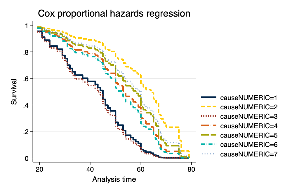
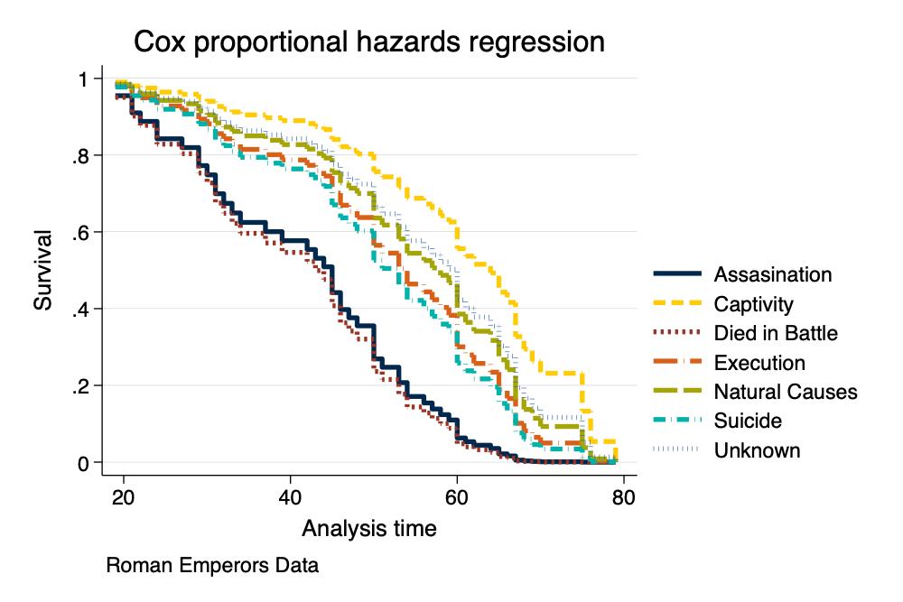
. stcurve, survival at(causeNUMERIC=(1(1)7)) ///
> scheme(michigan) // basic survival curve by causeNUMERIC
note: function evaluated at specified values of selected covariates and overall means
      of other covariates (if any).
. graph export mycox1.png, width(1000) replace
file
    /Users/agrogan/Desktop/GitHub/newstuff/categorical/survival-analysis-and-event-hi
    > story/emperors/mycox1.png saved as PNG format
. stcurve, survival ///
> at(causeNUMERIC=(1(1)7)) ///
> caption("Roman Emperors Data") ///
> legend(order(1 "Assasination" 2 "Captivity" 3 "Died in Battle" ///
> 4 "Execution" 5 "Natural Causes" 6 "Suicide" 7 "Unknown")) ///
> scheme(michigan) // more nicely formatted survival curve
note: function evaluated at specified values of selected covariates and overall means
      of other covariates (if any).
. graph export mycox2.png, width(1000) replace
file
    /Users/agrogan/Desktop/GitHub/newstuff/categorical/survival-analysis-and-event-hi
    > story/emperors/mycox2.png saved as PNG format
. estat phtest, detail // formal test of PH assumption

Test of proportional-hazards assumption

Time function: Analysis time
─────────────┬──────────────────────────────────────────
             │        rho     chi2       df    Prob>chi2
─────────────┼──────────────────────────────────────────
1.causeNUM~C │   -0.04848     0.17        1       0.6819
2.causeNUM~C │    0.00996     0.01        1       0.9397
3.causeNUM~C │    0.01796     0.02        1       0.8869
4.causeNUM~C │   -0.15154     1.62        1       0.2032
5b.causeNU~C │          .        .        1           .
6.causeNUM~C │   -0.31746    10.60        1       0.0011
7.causeNUM~C │    0.13799     1.11        1       0.2912
1.riseNUME~C │    0.18269     2.18        1       0.1399
2.riseNUME~C │    0.30901     8.28        1       0.0040
3.riseNUME~C │    0.10627     0.77        1       0.3790
4.riseNUME~C │    0.10649     0.95        1       0.3304
5b.riseNUM~C │          .        .        1           .
6.riseNUME~C │    0.12455     0.91        1       0.3402
7.riseNUME~C │    0.18581     2.10        1       0.1477
8.riseNUME~C │    0.23405     3.44        1       0.0638
─────────────┼──────────────────────────────────────────
 Global test │               21.90       13       0.0569
─────────────┴──────────────────────────────────────────
. stphplot, by(causeNUMERIC) scheme(michigan) // graphical test of PH assumption

        Failure _d: 1 (meaning all fail)
  Analysis time _t: age
. graph export ph.png, width(1000) replace
file
    /Users/agrogan/Desktop/GitHub/newstuff/categorical/survival-analysis-and-event-hi
    > story/emperors/ph.png saved as PNG format
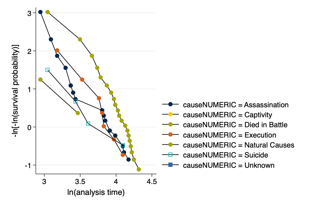
Had the proportional hazards assumption been violated, we could correct for this violation in one of two ways:
age) with the variable violating the assumption.e.g. stcox ib5.causeNUMERIC age#ib5.riseNUMERIC.
Note: In this relatively small sample this command fails to converge, perhaps because of sample size; or perhaps because there is no underlying violation of the proportional hazards assumption.
, strata(varname) option to stratify
on the variable violating the assumption.Note that the command below provides results, but does not provide parameter estimates for the variable on which we are stratifying,
riseNUMERIC.
. stcox ib5.causeNUMERIC, strata(riseNUMERIC)

        Failure _d: 1 (meaning all fail)
  Analysis time _t: age

Iteration 0:  Log likelihood = -110.21173
Iteration 1:  Log likelihood = -106.78694
Iteration 2:  Log likelihood = -106.44767
Iteration 3:  Log likelihood = -106.33876
Iteration 4:  Log likelihood = -106.30024
Iteration 5:  Log likelihood = -106.28627
Iteration 6:  Log likelihood = -106.28115
Iteration 7:  Log likelihood = -106.27928
Iteration 8:  Log likelihood = -106.27859
Iteration 9:  Log likelihood = -106.27833
Iteration 10: Log likelihood = -106.27824
Iteration 11: Log likelihood = -106.27821
Iteration 12: Log likelihood = -106.27819
Iteration 13: Log likelihood = -106.27819
Iteration 14: Log likelihood = -106.27819
Iteration 15: Log likelihood = -106.27819
Iteration 16: Log likelihood = -106.27819
Iteration 17: Log likelihood = -106.27819
Iteration 18: Log likelihood = -106.27819
Iteration 19: Log likelihood = -106.27819
Refining estimates:
Iteration 0:  Log likelihood = -106.27819
Iteration 1:  Log likelihood = -106.27819
Iteration 2:  Log likelihood = -106.27819
Iteration 3:  Log likelihood = -106.27819
Iteration 4:  Log likelihood = -106.27819
Iteration 5:  Log likelihood = -106.27819
Iteration 6:  Log likelihood = -106.27819
Iteration 7:  Log likelihood = -106.27819
Iteration 8:  Log likelihood = -106.27819
Iteration 9:  Log likelihood = -106.27819
Iteration 10: Log likelihood = -106.27819
Iteration 11: Log likelihood = -106.27819
Iteration 12: Log likelihood = -106.27819
Iteration 13: Log likelihood = -106.27819
Iteration 14: Log likelihood = -106.27819

Stratified Cox regression with Breslow method for ties
Strata variable: riseNUMERIC

No. of subjects =    61                                 Number of obs =     61
No. of failures =    61
Time at risk    = 2,984
                                                        LR chi2(6)    =   7.87
Log likelihood = -106.27819                             Prob > chi2   = 0.2480

────────────────┬────────────────────────────────────────────────────────────────
             _t │ Haz. ratio   Std. err.      z    P>|z|     [95% conf. interval]
────────────────┼────────────────────────────────────────────────────────────────
   causeNUMERIC │
 Assassination  │   2.055452   .7768999     1.91   0.057     .9798928    4.311578
     Captivity  │   2.30e-15   4.51e-08    -0.00   1.000            0           .
Died in Battle  │   1.888973   1.130025     1.06   0.288     .5848147    6.101451
     Execution  │   1.581336   .7416243     0.98   0.328        .6307     3.96484
       Suicide  │   1.130873    .808074     0.17   0.863     .2787286    4.588243
       Unknown  │   .8796497   .9202359    -0.12   0.902     .1131969    6.835731
────────────────┴────────────────────────────────────────────────────────────────
Johnson, L. L., & Shih, J. H. (2007). CHAPTER 20 - An Introduction to Survival Analysis (J. I. Gallin & F. P. Ognibene, eds.). https://doi.org/https://doi.org/10.1016/B978-012369440-9/50024-4
failvair is often something like
died.↩︎