Introduction

Below you will find a simulated data set that might help you think about constructing a data set for survival analysis, or event history analysis.

These simulated data represent a common situation in which a categorical status (like a diagnosis of depression or PTSD) is observed at different time points.

An event is defined as a (relatively sudden) change from a status of 0 to a status of 1.

These data are in wide format. We will need to think differently if data are in long format.

Get The Data

. clear all

. use "simulated-survival-data.dta", clear

In this example, we are going to think about how to take a data set of statuses and turn it into a data set of events.

Look At The Data

Notice how this is a wide data set. Every individual has a single row of data, and information on status at each of the timepoints is contained in the same row.

. list

     ┌──────────────────────────────────┐
     │ id   status1   status2   status3 │
     ├──────────────────────────────────┤
  1. │  1         0         0         0 │
  2. │  2         0         1         1 │
  3. │  3         0         0         1 │
     └──────────────────────────────────┘

Notice How Individual Status Changes Over Time.

1. Status never changes for individual 1. The event never occurs for individual 1. Individual 1’s event time is therefore censored.
2. Status changes at wave 2 for individual 2. The event therefore occurs for individual 2 at wave 2. Individual 2’s event time is therefore observed.
3. Status changes at wave 3 for individual 3. The event is therefore conceptualized as occurring for individual 3 at wave 3. Individual 3’s event time is therefore observed.

How Do We Turn This Data Set Into A Data Set of Event Times?

First, we want to make sure that it is appropriate to conceptualize this data set of individuals as a data set for whom the event has not yet occurred.

Second, we want to create an event time out of these status changes.

Our code might look something as follows.

I am assuming in the code below that waves are 1 year apart, and you might want to adjust your code accordingly if waves are differentially spaced.

Generate an Event Time

. * possibly... only keep observations with nonmissing statuses

. keep if status1 != . & status2 != .
(0 observations deleted)

. * initialize to longest time

. * censored observations will have the value of the longest possible event time

. generate event_time = 3

. * change event time to 2 if status2 == 2
. * change event time to 1 if status1 == 1

. * notice that I am doing this in *reverse* order
. * to capture the earliest event time

. replace event_time = 2 if status2 == 1 // event time is 2 if status 2 is 1
(1 real change made)

. replace event_time = 1 if status1 == 1 // event time is 1 if status 1 is 1
(0 real changes made)

Generate A Failure (Censoring) Indicator

. * failure becomes 1 for those 
. * for whom event occurred at some timepoint

. generate failure = 0 // initialize

. * change failure to 1 if any status variable == 1

. replace failure = 1 if status1 == 1 | status2 == 1 | status3 == 1 
(2 real changes made)

You can see that our data now have an event time, and a censoring status.

. list, abbreviate(10) // list out the data

     ┌─────────────────────────────────────────────────────────┐
     │ id   status1   status2   status3   event_time   failure │
     ├─────────────────────────────────────────────────────────┤
  1. │  1         0         0         0            3         0 │
  2. │  2         0         1         1            2         1 │
  3. │  3         0         0         1            3         1 │
     └─────────────────────────────────────────────────────────┘

stset the data

Inspection of the results from the stset command indicates that the data appears to have been stset correctly.

. stset event_time, failure(failure == 1)

Survival-time data settings

         Failure event: failure==1
Observed time interval: (0, event_time]
     Exit on or before: failure

──────────────────────────────────────────────────────────────────────────
          3  total observations
          0  exclusions
──────────────────────────────────────────────────────────────────────────
          3  observations remaining, representing
          2  failures in single-record/single-failure data
          8  total analysis time at risk and under observation
                                                At risk from t =         0
                                     Earliest observed entry t =         0
                                          Last observed exit t =         3

Graph of Survival Function

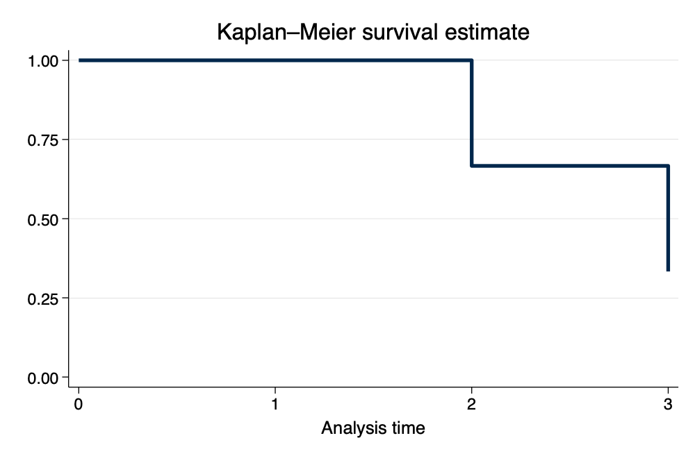
. sts graph, scheme(michigan)

        Failure _d: failure==1
  Analysis time _t: event_time

. graph export simulated-survival-data.png, width(1000) replace
file
    /Users/agrogan/Desktop/GitHub/newstuff/categorical/survival-analysis-and-event-hi
    > story/simulated-survival-data.png saved as PNG format

Notice how the graph makes intuitive sense if we consider the combination of event_time and failure for each observation.