Background 🌲

In web slide versions of this material press b for bigger text and s for smaller text.

Chihara and Hesterberg (2018) provide a data set concerning the growth of Black Spruce Trees. According to these authors:

“Black spruce (Picea mariana) is a species of a slow-growing coniferous tree found across the northern part of North America. It is commonly found on wet organic soils. In a study conducted in the 1990s, a biologist interested in factors affecting the growth of the black spruce planted its seedlings on sites located in boreal peatlands in northern Manitoba, Canada (Camil et al. (2010)). The data set Spruce contains a part of the data from the study (Table 1.8). Seventy-two black spruce seedlings were planted in four plots under varying conditions (fertilizer–no fertilizer, competition–no competition), and their heights and diameters were measured over the course of 5 years. The researcher wanted to see whether the addition of fertilizer or the removal of competition from other plants (by weeding) affected the growth of these seedlings.”

The Research Question 🌲

We are going to consider the potentially causal estimate of the effect of fertilizer on tree height at year 5. Along the way we will give brief attention to the advantages and disadvantages of each approach. Because of the research design, we have strong reasons to consider fertilizer as having a causal effect on tree height but we will nonetheless explore this question using a variety of statistical models.

A secondary purpose of this document is to demonstrate that Stata syntax makes it easy to test and compare multiple statistical models because of the uniform Stata syntax, which is almost always: command variable(s), options.

Causality 🌲

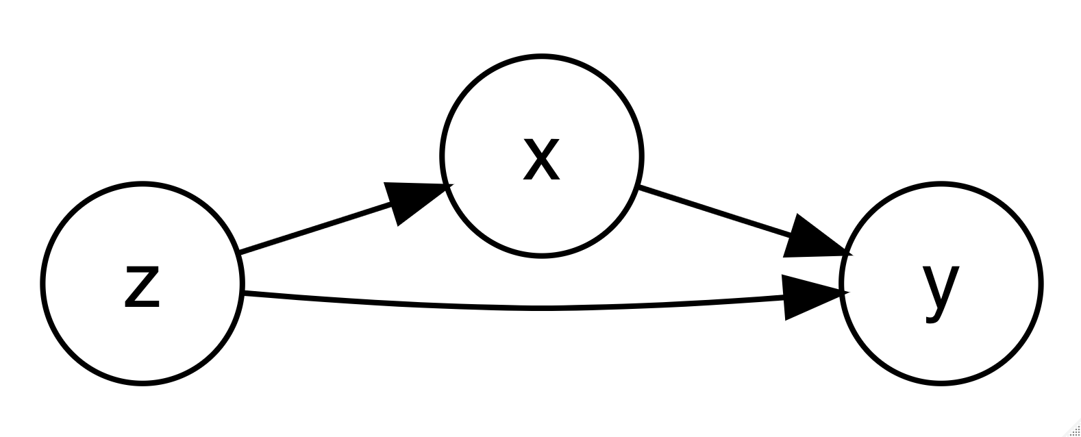
A variable \(x\) can only be considered to have causal association with \(y\) if the following conditions are met (Holland, 1986):

1. \(x\) is correlated with \(y\).
2. \(x\) precedes \(y\) in time order.
3. The association between \(x\) and \(y\) can not be accounted for by any third variable \(z\).

Hence, for this particular data, we are exploring:

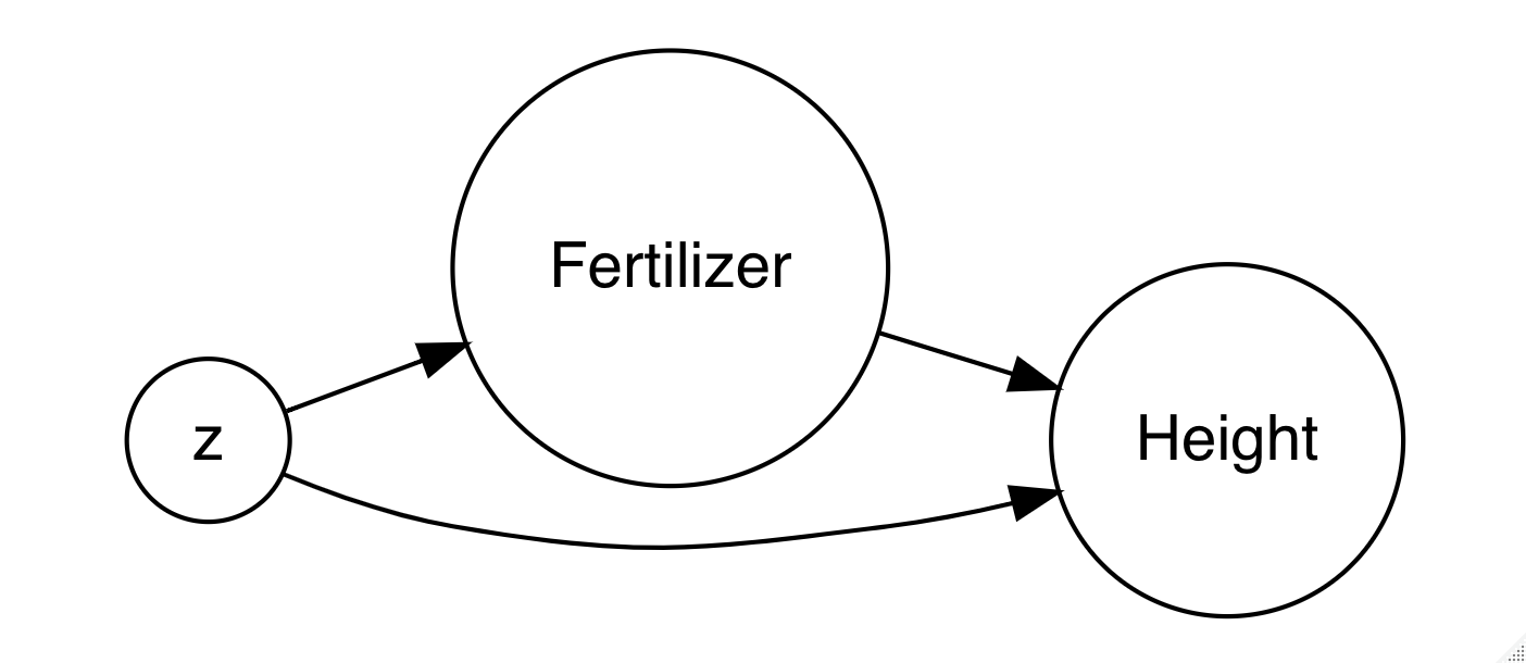
What happens to the association of fertilizer and tree height when we control for possible confounding variables \(z\) using various statistical strategies?

(For more interactive exploration of these ideas, see this demo).

Setup 🌲

Get Data

. clear all

.         
. use spruce.dta, clear

Dataset Description

. describe    

Contains data from spruce.dta
 Observations:            72                  
    Variables:             9                  26 Apr 2020 12:18
────────────────────────────────────────────────────────────────────────────────────────────
Variable      Storage   Display    Value
    name         type    format    label      Variable label
────────────────────────────────────────────────────────────────────────────────────────────
Tree            long    %12.0g                Tree number
Competition     long    %12.0g     Competition
                                              C (competition), CR (competition removed)
Fertilizer      long    %12.0g     Fertilizer
                                              F (fertilized), NF (not fertilized)
Height0         double  %10.0g                Height (cm) of seedling at planting
Height5         double  %10.0g                Height (cm) of seedling at year 5
Diameter0       double  %10.0g                Diameter (cm) of seedling at planting
Diameter5       double  %10.0g                Diameter (cm) of seedling at year 5
Ht_change       double  %10.0g                Change (cm) in height
Di_change       double  %10.0g                Change (cm) in diameter
────────────────────────────────────────────────────────────────────────────────────────────
Sorted by: 
     Note: Dataset has changed since last saved.

Spruce Data And Causal Criteria 🌲

Let’s consider in turn each of the criteria for causality.

1. Empirically, fertilizer is correlated with tree height.

2. From the research design, we know that fertilizer comes prior to tree height at year 5.
3. We are going to use various statistical strategies–detailed below–to assess whether the association of fertilizer and tree height can be accounted for by any third variable.

Analyses 🌲

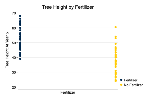
t Test (ttest y, by(x))

A t test compares the difference between the means of two groups to the standard error of the difference between means.

Formally, \(t = \frac{\bar{x}_2 - \bar{x}_1}{s}\) where s is the standard error of the estimate of the mean.

More colloquially, the t test compares the differences between the two groups in standard error units.

A t test does not control for any additional variable(s).

. ttest Height5, by(Fertilizer)

Two-sample t test with equal variances
─────────┬────────────────────────────────────────────────────────────────────
Variable │     Obs        Mean    Std. err.   Std. dev.   [95% conf. interval]
─────────┼────────────────────────────────────────────────────────────────────
       F │      36    52.89167    1.396079    8.376476    50.05747    55.72586
      NF │      36    38.11944    1.465226    8.791354    35.14488    41.09401
─────────┼────────────────────────────────────────────────────────────────────
Combined │      72    45.50556    1.333392    11.31421    42.84685    48.16426
─────────┼────────────────────────────────────────────────────────────────────
    diff │            14.77222    2.023839                 10.7358    18.80864
─────────┴────────────────────────────────────────────────────────────────────
    diff = mean(F) - mean(NF)                                     t =   7.2991
H0: diff = 0                                     Degrees of freedom =       70

    Ha: diff < 0                 Ha: diff != 0                 Ha: diff > 0
 Pr(T < t) = 1.0000         Pr(|T| > |t|) = 0.0000          Pr(T > t) = 0.0000

The association of fertilizer with tree height is -14.77.

OLS Regression (regress y x1 x2 x3)

A regression estimates the association of a 1 unit change in each of the independent variables with change in the dependent variable, while accounting for all of the other independent variables in the model.

\(y_i = \beta_0 + \beta_1 x_{1i} + \Sigma \beta_k x_{ki} + e_i\)

Here \(x_{1i}\) is the treatment variable of interest.

A regression controls for the additional observed variables (\(x_{ki}\)) that are included in the model.

. regress Height5 Fertilizer Height0 Competition

      Source │       SS           df       MS      Number of obs   =        72
─────────────┼──────────────────────────────────   F(3, 68)        =     50.97
       Model │  6291.23189         3   2097.0773   Prob > F        =    0.0000
    Residual │  2797.56589        68  41.1406748   R-squared       =    0.6922
─────────────┼──────────────────────────────────   Adj R-squared   =    0.6786
       Total │  9088.79778        71  128.011236   Root MSE        =    6.4141

─────────────┬────────────────────────────────────────────────────────────────
     Height5 │ Coefficient  Std. err.      t    P>|t|     [95% conf. interval]
─────────────┼────────────────────────────────────────────────────────────────
  Fertilizer │  -14.71947   1.511991    -9.74   0.000    -17.73661   -11.70234
     Height0 │   .8631456    .374817     2.30   0.024       .11521    1.611081
 Competition │   10.52346    1.52143     6.92   0.000      7.48749    13.55942
       _cons │   39.22163   6.189971     6.34   0.000     26.86974    51.57353
─────────────┴────────────────────────────────────────────────────────────────

The association of fertilizer with tree height is -14.72.

Propensity Scores (teffects psmatch (y) (t x1 x2))

The propensity score uses a logistic regression to estimate the predicted probability of being administered the treatment (t in the above syntax), in this example, fertilizer. Treatment observations are matched to the most similar comparison group observation in terms of this probability, and an average difference is calculated.

A propensity score analysis controls for the additional observed variables that are included in the model.

. teffects psmatch (Height5) (Fertilizer Height0 Competition)

Treatment-effects estimation                   Number of obs      =         72
Estimator      : propensity-score matching     Matches: requested =          1
Outcome model  : matching                                     min =          1
Treatment model: logit                                        max =          3
─────────────┬────────────────────────────────────────────────────────────────
             │              AI robust
     Height5 │ Coefficient  std. err.      z    P>|z|     [95% conf. interval]
─────────────┼────────────────────────────────────────────────────────────────
ATE          │
  Fertilizer │
  (NF vs F)  │  -12.71019   1.988531    -6.39   0.000    -16.60763   -8.812737
─────────────┴────────────────────────────────────────────────────────────────

The association of fertilizer with tree height is -12.71.

Assess Balance of Propensity Score Model

With many thanks to Jorge Cuartas for ideas for some of this code.

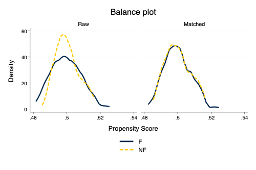
. tebalance summarize
(refitting the model using the generate() option)

Covariate balance summary

                         Raw      Matched
─────────────────────────────────────────
Number of obs =           72          144
Treated obs   =           36           72
Control obs   =           36           72
─────────────────────────────────────────

────────────────┬────────────────────────────────────────────────
                │Standardized differences          Variance ratio
                │        Raw     Matched           Raw    Matched
────────────────┼────────────────────────────────────────────────
        Height0 │  -.0296893    .0392505      .6061612   .9203723
    Competition │          0    .2795331             1   1.048701
────────────────┴────────────────────────────────────────────────

. tebalance density, scheme(michigan)
(refitting the model using the generate() option)

. 
. graph export mydensity.png, width(500) replace
file /Users/agrogan/Desktop/GitHub/teaching/spruce/mydensity.png saved as PNG format

References 🌲

Camill, P., Chihara, L., Adams, B., Andreassi, C., Barry, A. N. N., Kalim, S., … Rafert, G. (2010). Early life history transitions and recruitment of Picea mariana in thawed boreal permafrost peatlands. Ecology. https://doi.org/10.1890/08-1839.1

Chihara, L. M., & Hesterberg, T. C. (2018). Mathematical Statistics with Resampling and R. https://doi.org/10.1002/9781119505969

Holland, P. W. (1986). Statistics and Causal Inference. Journal of the American Statistical Association, 81(396), 945–960. https://doi.org/10.1080/01621459.1986.10478354