Workflow
1 Introduction
I have increasingly been thinking about the idea of workflow in data science / data analysis work.
So many workflows follow the same conceptual pattern.
2 Visually and Conceptually
%%{
  init: {
    'theme': 'base',
    'themeVariables': {
      'primaryColor': '#FFCB05',
      'primaryTextColor': '#000000',
      'primaryBorderColor': '#00274C',
      'lineColor': '#00274C',
      'secondaryColor': '#00274C',
      'secondaryTextColor': '#000000',
      'tertiaryColor': '#F2F2F2',
      'tertiaryBorderColor': '#00274C'
    }
  }
}%%

flowchart TB

ask[ask a question]-->open

open[open the raw data]-->keep

keep[select or keep variables]-->clean

clean[clean the data, e.g. outliers & errors]-->wrangle

wrangle[create any new variables or scales]-->descriptives

descriptives[descriptive statistics]-->visualize

visualize[visualize the data]-->analyze

analyze[analyze with bivariate or multivariate statistics]-->share["share your results with your community(ies)"]
3 Characteristics of Good Workflows
Increasingly, we want to think about workflows that are
- documentable, transparent, and auditable: We have a record of what we did if we want to double check our work, clarify a result, or develop a new project with a similar process. We, or others, can find the inevitable errors in our work, and correct them.
- replicable: Others can replicate our findings with the same or new data.
- scalable: We are developing a process that can be as easily used with thousands or millions of rows of data as it can with ten rows of data. We are developing a process that can be easily repeated if we are constantly getting new or updated data, e.g. getting new data every week, or every month.
4 Complex Workflows
For complex workflows, we will often want to write a script or code.
The more graphs or calculations I have to make, the more complex the project, the more the desires of the community or client are likely to change, the more frequently the data is being updated, the more team members that are involved in the workflow, and/or the more mission critical the results (i.e. I need auditability, documentation, and error correction) the more likely I am to use a scripting or coding tool like Stata or R.
| Simple Process: Single Graph or Calculation | Complex Process: Multiple Graphs or Calculations. | |
|---|---|---|
| Process Run Only Once | Spreadsheet: Excel or Google | Scripting Tool: Stata or R |
| Process Run Multiple Times (Perhaps As Data Are Regularly Updated) | Scripting Tool: Stata or R | Scripting Tool: Stata or R |
5 Best Practices
Always (or usually) beginning with the raw data, and then writing and running a script or code that generates our results allows us to develop a process that is documentable, auditable, replicable and scalable.
It is usually best to store quantitative data in a statistical format such as R, Stata, or SPSS. Spreadsheets are likely to be a bad tool for storing quantitative data.
It is also very important to be aware that good complex workflows are highly iterative and highly collaborative, often requiring a lot of conversation. Some–hopefully small–amount of error is unavoidable and inevitable. Good complex workflows require a safe workspace in which team members feel free to talk through their ideas, admit their own errors, and help with others’ mistakes in a non-judgmental fashion. Such a safe environment is necessary to build an environment where the overall error rate is low.
Developing a good documented and auditable workflow that is implemented in code requires a lot of patience, and often, many iterations. Working through these many iterations can be psychologically demanding. It is important to remember that careful attention to getting the details right early in the research process, while sometimes tiring and frustrating, will pay large dividends later on when the research is reviewed, presented, published and read.
6 Example
Below is an example that uses the Palmer Penguins data set.
The example below is in Stata, due to Stata’s ease of readability, but could as easily be written in any other language that has scripting, such as SPSS, SAS, R, or Julia.
* Learning About Penguins

* Ask A Question

* What can I learn about penguins?
* Open The Raw Data

use "https://github.com/agrogan1/Stata/raw/main/do-files/penguins.dta", clear

* Clean and Wrangle Data

generate big_penguin = body_mass_g > 4000 // create a big penguin variable
* Descriptive Statistics

use "https://github.com/agrogan1/Stata/raw/main/do-files/penguins.dta", clear

dtable culmen_length_mm culmen_depth_mm flipper_length_mm body_mass_g i.species
Summary
-------------------------------------
N 344
culmen_length_mm 43.922 (5.460)
culmen_depth_mm 17.151 (1.975)
flipper_length_mm 200.915 (14.062)
body_mass_g 4,201.754 (801.955)
species
Adelie 152 (44.2%)
Chinstrap 68 (19.8%)
Gentoo 124 (36.0%)
-------------------------------------
* Visualize The Data
use "https://github.com/agrogan1/Stata/raw/main/do-files/penguins.dta", clear
graph bar body_mass_g, over(species) // bar graph
quietly graph export "mybargraph.png", replace
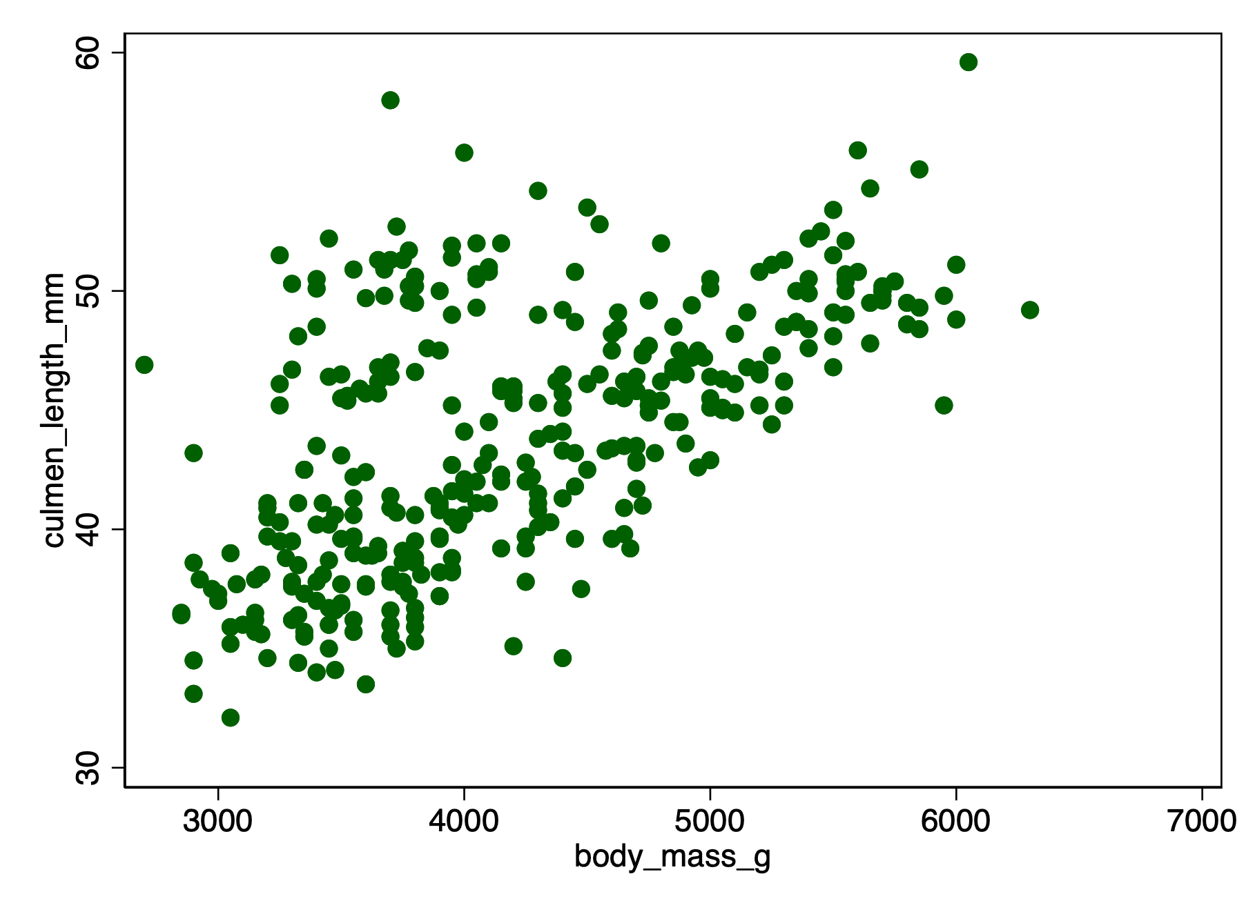
twoway scatter culmen_length_mm body_mass_g // scatterplot
quietly graph export "myscatterplot.png", replace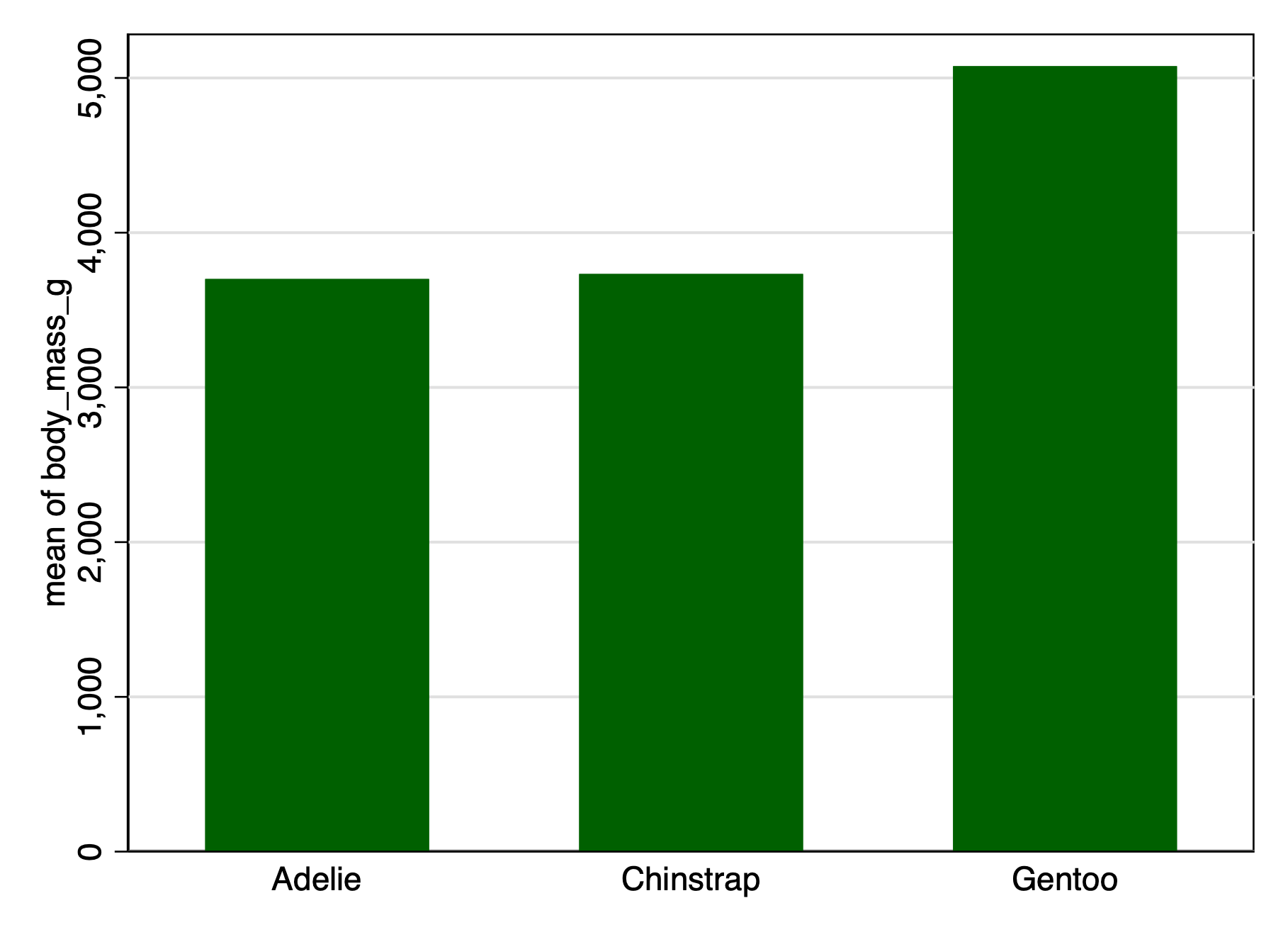
* Analyze

use "https://github.com/agrogan1/Stata/raw/main/do-files/penguins.dta", clear

quietly: regress culmen_length_mm body_mass_g // regress culmen length on body mass

estimates store M1 // store these estimates

etable, estimates(M1) showstars showstarsnote // nice table of estimates
culmen_length_mm
---------------------------------------
body_mass_g 0.004 **
(0.000)
Intercept 26.899 **
(1.269)
Number of observations 342
---------------------------------------
** p<.01, * p<.057 Multiple Person Workflows
When workflows involve multiple people, all of the above considerations apply, but the situation often becomes more complex. Two hypothetical multiple person workflows are illustrated below.
In the diagram below, one workflow is uncoordinated. Each person’s work is not available to the others, which may cause difficulties if people’s work is supposed to build on the work of others. If one team member makes updates or corrects errors, the results of these efforts are not automatically available to the others.
In contrast, in the diagram below, one workflow is coordinated. Each person’s work is available to the others so that updates and corrections to errors are propagated through the workflow, and into final analyses and visualizations.
It is often the case that a coordinated workflow requires more coordination, time, energy, and patience to implement than an uncoordinated workflow, but a coordinated workflow is likely to pay benefits in terms of all of the advantages of good workflows listed above.
%%{
  init: {
    'theme': 'base',
    'themeVariables': {
      'primaryColor': '#FFCB05',
      'primaryTextColor': '#000000',
      'primaryBorderColor': '#00274C',
      'lineColor': '#00274C',
      'secondaryColor': '#00274C',
      'secondaryTextColor': '#000000',
      'tertiaryColor': '#F2F2F2',
      'tertiaryBorderColor': '#00274C'
    }
  }
}%%

flowchart TB

%% first block: Uncoordinated Workflow

rawdataA[raw data]

rawdataB[raw data]

person1A[person 1]

person1B[person 1]

cleandataA[cleans the data]

cleandataB[cleans the data]

person2A[person 2]

person2B[person 2]

scale1A[creates scale 1]

scale1B[creates scale 1]

person3A[person 3]

person3B[person 3]

scale2A[creates scale 2]

scale2B[creates scale 2]

person4A[person 4]

person4B[person 4]

complexanalysisA[complex analysis <br>and visualization]

complexanalysisB[complex analysis <br>and visualization]

subgraph "UNCOORDINATED Workflow"

direction TB

rawdataA-->person1A

person1A-->cleandataA

rawdataA-->person2A

person2A-->scale1A

rawdataA-->person3A

person3A-->scale2A

rawdataA-->person4A

person4A-->complexanalysisA

end

subgraph "COORDINATED Multiperson Workflow"

direction TB

rawdataB-->person1B

person1B-->cleandataB

cleandataB-->person2B

person2B-->scale1B

scale1B-->person3B

person3B-->scale2B

scale2B-->person4B

person4B-->complexanalysisB

end