Bayesian Calculations: Simulation of Coin Flipping

Prior With 3 Values; Data on Coin Flips; Likelihood and Posterior

1 Background

Bayes Theorem allows us to state our prior beliefs, to calculate the likelihood of our data given those beliefs, and then to update those beliefs with data, thus arriving at a set of posterior beliefs. However, Bayesian calculations can be difficult to understand. This document attempts to provide a simple walkthrough of some Bayesian calculations.

library(pander) # nice tables

library(tibble) # data frames

library(ggplot2) # beautiful graphs

2 Bayes Rule

Mathematically Bayes Theorem is as follows:

\[P(H|D) = \frac{P(D|H)P(H)}{P(D)} \tag{1}\]

In words, Bayes Theorem may be written as follows:

\[\text{posterior} = \frac{\text{likelihood} \times \text{prior}}{\text{data}} \tag{2}\]

Our posterior beliefs are proportional to our prior beliefs, multiplied by the likelihood of those beliefs, given the data.

3 This Example

In this example, we provide an example of using Bayes Theorem to examine our conclusions about the proportion of heads when a coin is flipped 10 times.

Conventionally, we call this proportion that we are trying to estimate \(\theta\).

For the sake of simplicity, this example uses a relatively simple set of prior beliefs about 3 possible values for the proportion \(\theta\).

R code in this example is adapted and simplified from Kruschke (2011), p. 70

4 Prior

We set a simple set of prior beliefs, concerning 3 values of \(\theta\), the proportion of heads.

theta1 <- c(.25, .50, .75) # candidate parameter values

ptheta1 <- c(.25, .50, .25) # prior probabilities

ptheta1 <- ptheta1/sum(ptheta1) # normalize

Our values of \(\theta\) are 0.25, 0.5 and 0.75, with probabilities \(P(\theta)\) of 0.25, 0.5 and 0.25.

ggplot(data = NULL,
       aes(x = theta1,
           y = ptheta1)) +
  geom_bar(stat = "identity", 
           fill = "#FFBB00") +
  labs(title = "Prior Probabilities") +
  theme_minimal()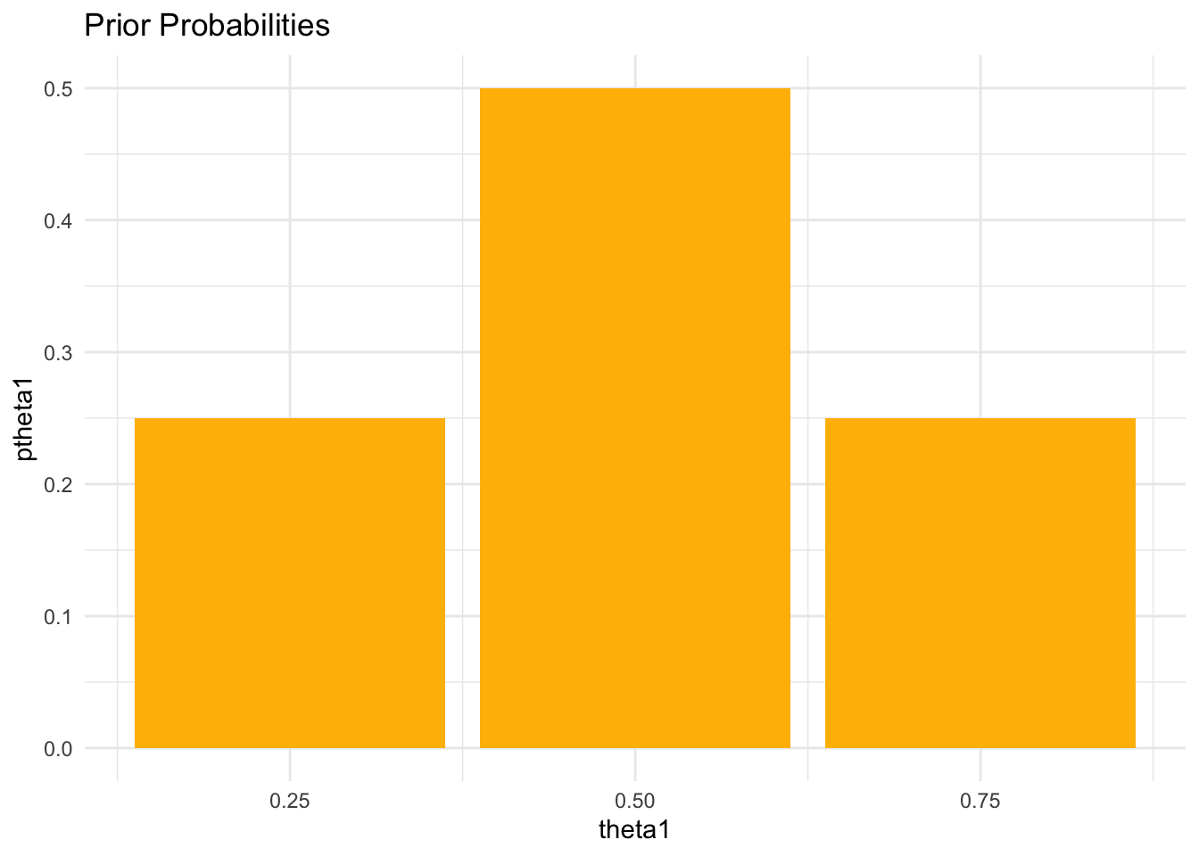

myBayesianEstimates <- tibble(theta1, ptheta1) # data frame

pander(myBayesianEstimates) # nice table

theta1	ptheta1
0.25	0.25
0.5	0.5
0.75	0.25

5 The Data

10 coin flips. 1 Heads. 9 Tails.

data1 <- c(1, 0, 0, 0, 0, 0, 0, 0, 0, 0) # the data

data1_factor <- factor(data1,
                       levels = c(0, 1),
                       labels = c("T", "H"))

n_heads <- sum(data1 == 1) # number of heads

n_tails <- sum(data1 == 0) # number of tails

x <- seq(1, 10) # x goes from 1 to 10

y <- rep(1, 10) # y is a sequence of 10 1's

coindata <- data.frame(x, y, data1_factor) # data for visualization

ggplot(coindata,
       aes(x = x,
           y = y,
           label = data1_factor,
           color = data1_factor)) +
  geom_point(size = 10, pch = 1) +
  geom_text() +
  labs(x = "",
       y = "") +
  scale_color_manual(values = c("black", "red")) +
  theme_void() +
  theme(legend.position = "none")

6 Likelihood

The likelihood is the probability that a given value of \(\theta\) would produce this number of heads.

The probability of multiple independent events \(A\), \(B\), \(C\), etc. is \(P(A, B, C, ...) = P(A) \times P(B) \times P(C) \times ...\).

Therefore, in this case, the likelihood is proportional to \([P(heads)]^{\text{number of heads}}\) and multiply this by \([P(tails)]^{\text{number of tails}}\).

Thus:

\[\mathcal{L}(\theta) \propto \theta^{\text{number of heads}} \times (1-\theta)^{\text{number of tails}}\]

likelihood1 <- theta1^n_heads * (1 - theta1)^n_tails # likelihood

ggplot(data = NULL,
       aes(x = theta1,
           y = likelihood1)) +
  geom_bar(stat = "identity", 
           fill = "#375E97") +
  labs(title = "Likelihood") +
  theme_minimal()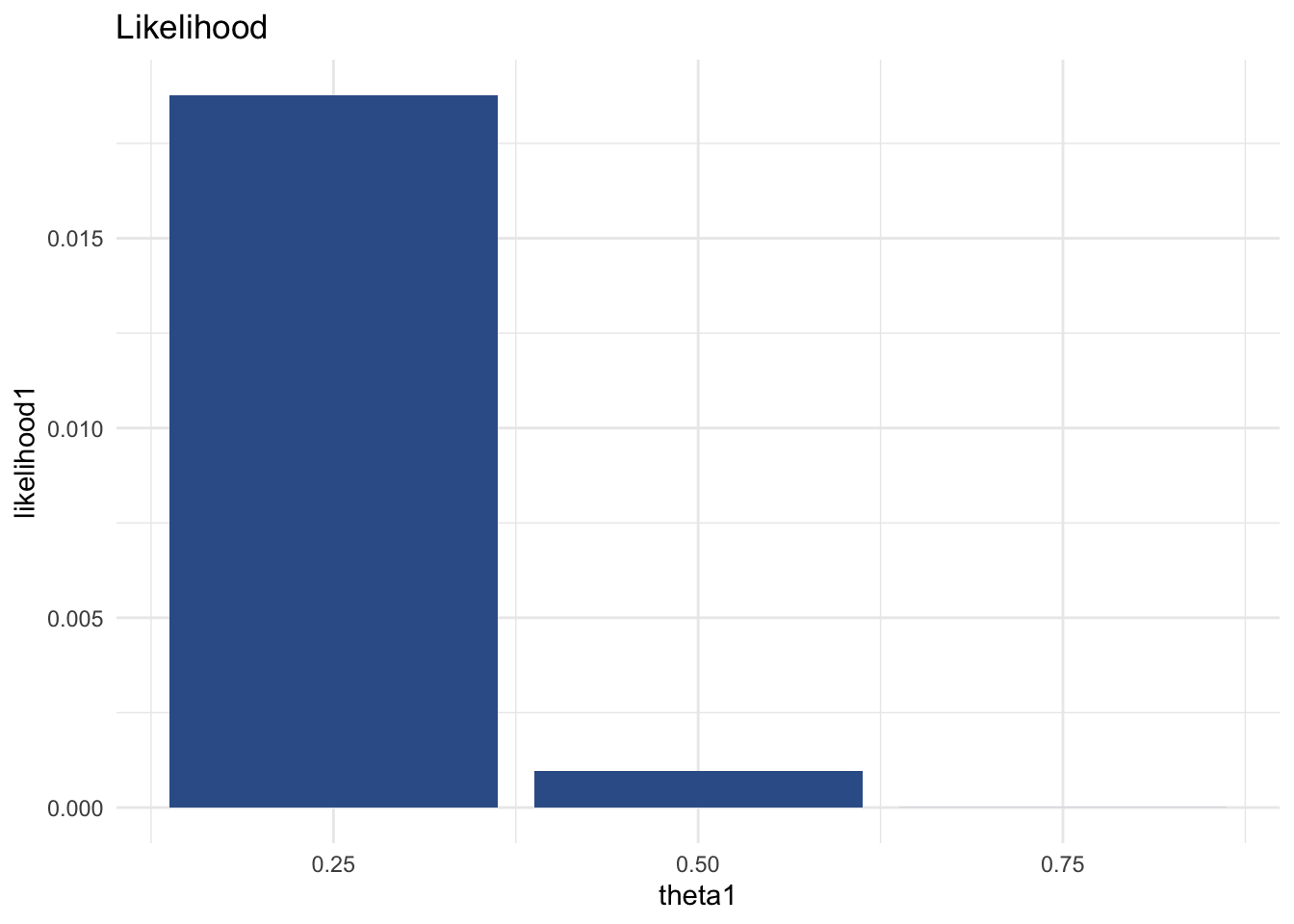

At this point our estimates include not only a value of \(\theta\) and \(P(\theta)\), but also the likelihood, \(\mathcal{L}(\theta)\).

myBayesianEstimates <- tibble(theta1, ptheta1, likelihood1)

pander(myBayesianEstimates) # nice table

theta1	ptheta1	likelihood1
0.25	0.25	0.01877
0.5	0.5	0.0009766
0.75	0.25	2.861e-06

7 Posterior

We then calculate the denominator of Bayes theorem:

\[\Sigma [\mathcal{L}(\theta) \times P(\theta)]\]

pdata1 <- sum(likelihood1 * ptheta1) # normalize

We then use Bayes Rule to calculate the posterior:

\[P(H|D) = \frac{P(D|H)P(H)}{P(D)}\]

posterior1 <- likelihood1 * ptheta1 / pdata1 # Bayes Rule

ggplot(data = NULL,
       aes(x = theta1,
           y = posterior1)) +
  geom_bar(stat = "identity", 
           fill = "#3F681C") +
  labs(title = "Posterior") +
  theme_minimal()

Our estimates now include \(\theta\), \(P(\theta)\), \(\mathcal{L}(\theta)\) and \(P(\theta | D)\).

myBayesianEstimates <- tibble(theta1, ptheta1, likelihood1, posterior1)

pander(myBayesianEstimates) # nice table

theta1	ptheta1	likelihood1	posterior1
0.25	0.25	0.01877	0.9056
0.5	0.5	0.0009766	0.09423
0.75	0.25	2.861e-06	0.000138

Estimates Are A Combination of Prior and Likelihood

Notice how \(\theta = .5\) has the highest prior probability. \(\theta = .25\) has the highest likelihood. \(\theta = .75\) has an equivalent prior probability to \(\theta = .25\) but a much lower likelihood. The posterior is proportional to the prior multiplied by the likelihood. In this case the posterior estimates strongly favor \(\theta = .25\).

8 Credits

Prepared by Andy Grogan-Kaylor agrogan@umich.edu, https://agrogan1.github.io/.

Questions, comments and corrections are most welcome.