A Discussion Focused, Collaborative, Lab-Based Introduction to Bayesian Statistics
Thinking about Bayesian analysis can be HARD. Doing Bayesian analysis can be EASY! ‘Fail Frequently! Fail Forward!’
2023-10-27
Navigation
- o for outline
- f for full screen
- Alt-Click to zoom
- Scroll ⇩ to the bottom of each column of slides; then ⇨
- Grey slides represent topics we most likely will not cover in detail, but are included for the sake of completeness, and will be covered if time allows.
Beginning (10 Minutes)
Background

Bayesian statistics are often touted as the new statistics, that should perhaps supplant traditional frequentist statistics.
Advantages
Bayesian statistics have the advantage of being able to incorporate prior information (e.g. clinical wisdom & insight, community knowledge, results of meta-analyses and literature reviews).
Bayesian statistics also have the advantage that we are not simply deciding whether to reject the null hypotheses, \(P(D|H_0)\) but are rather able to evaluate the probability of a hypothesis, \(P(H|D)\). In essence, this means that we can sometimes decide to accept the null hypothesis, rather than failing to reject the null hypothesis.
Disadvantages
However, Bayesian statistics may be very difficult to understand. Further, while statistical software for Bayesian inference is becoming easier and easier to use, syntax for Bayesian inference may remain complicated and counter-intuitive. Bayesian models may take a long time to run.
Lastly, the advantages of being able to incorporate prior information and to accept the null hypothesis may be overstated: prior information may be difficult to come by; and social science may be able to move forward quite well without the ability to accept null hypotheses.
In this presentation I hope to at least introduce some of these ideas, and to generate some discussion of them.
Bayes’ Theorem As Equation & Words (10 Minutes)
10 minutes is far too short a time to talk about how the mathematics of Bayes’ theorem imply, and connect to, all of the ideas that we will discuss in this presentation. Nevertheless, a presentation on Bayesian statistics would be incomplete without some reference to Bayes’ theorem. In this presentation, we gesture quickly at Bayes’ theorem to demonstrate that Bayes’ theorem contains at least two key ideas: We are estimating the probability of hypotheses; and we are using prior information. Discussion in later slides will connect us back to some of these ideas.
Equation
\[P(H|D) = \frac{P(D|H) P(H)}{P(D)}\]
Words
\[\text{posterior} = \frac{\text{likelihood} \times \text{prior}}{\text{data}}\]
\[\text{posterior} \propto \text{likelihood} \times \text{prior}\]
In Even More Words:
Our posterior (updated) beliefs about the probability of some hypothesis are proportional to our prior beliefs about the probability of that hypothesis multiplied by the likelihood that were our hypothesis true it would have generated the data we observe.
Why Do We Care / Should We Care? (40 Minutes Total)
Prior Information (20 Minutes)
Accepting The Null Hypothesis (20 Minutes, If Time)
We’ll likely circle back to this after running some analysis.
In Bayesian analysis, we are not assessing the plausibility of the data (\(P(D|H)\)), given the assumption of a null hypothesis \(H_0: \text{parameter value} = 0\). This feature of Bayesian analysis has a few key implications:
We are actually estimating–the probability of a particular hypothesis given the data–what we often think we are estimating in Frequentist analysis. Thus, after conducting a Bayesian analysis, we can simply say, “The probability of our hypothesis (\(P(H|D)\)) given the data is x,” rather than engaging in complicated statements about “Were the null hypothesis to be true, we estimate that it is p likely that we would see data as extreme, or more extreme, than we actually observed.”
Because we are directly estimating the probability of hypotheses, we can not only evaluate the probability of the null hypothesis (\(H_0\)), but also accept the null hypothesis (\(H_0\)), something that we are never supposed to be able to do in frequentist analysis. Being able to accept the null hypothesis may have implications for equivalency testing and theory simplification and may reduce publication bias, if we are not always looking for ways to reject \(H_0\).
https://agrogan1.github.io/Bayes/accepting-H0/accepting-H0.html
Lab and Questions (Stata) (Work At Your Own Pace and Leave When You’re Done) (Last 60 Minutes)
Thinking through Bayes is hard. We perhaps learn best by doing.
Our Data
We are using simulated data from my text on multilevel modeling, Multilevel Thinking: https://agrogan1.github.io/multilevel-thinking/simulated-multi-country-data.html.
This simulated data comes from multiple countries so we use mixed instead of regress to account for the clustering. However, our process would be largely the same if we were to use regress.
Basic Bayesian Regression
What do the results say (particularly about HDI)?
note: Gibbs sampling is used for regression coefficients and variance components.

Burn-in 2500 aaaaaaaaa1000aaaaaaaaa2000aaaaa done
Simulation 10000 .........1000.........2000.........3000.........4000.........5000.....
> ....6000.........7000.........8000.........9000.........10000 done

Multilevel structure
------------------------------------------------------------------------------
country
    {U0}: random intercepts
------------------------------------------------------------------------------

Model summary
-------------------------------------------------------------------------------------
Likelihood:
  outcome ~ normal(xb_outcome,{e.outcome:sigma2})

Priors:
  {outcome:physical_punishment warmth HDI _cons} ~ normal(0,10000)                (1)
                                            {U0} ~ normal(0,{U0:sigma2})          (1)
                              {e.outcome:sigma2} ~ igamma(.01,.01)

Hyperprior:
  {U0:sigma2} ~ igamma(.01,.01)
-------------------------------------------------------------------------------------
(1) Parameters are elements of the linear form xb_outcome.

Bayesian multilevel regression                          MCMC iterations  =     12,500
Metropolis–Hastings and Gibbs sampling                  Burn-in          =      2,500
                                                        MCMC sample size =     10,000
Group variable: country                                 Number of groups=        30
                                                        Obs per group:
                                                              min =        100
                                                              avg =      100.0
                                                              max =        100
                                                        Number of obs    =      3,000
                                                        Acceptance rate  =      .8149
                                                        Efficiency:  min =     .01661
                                                                     avg =      .5378
Log marginal-likelihood                                              max =          1

-------------------------------------------------------------------------------------
                    |                                                Equal-tailed
                    |      Mean   Std. dev.     MCSE     Median  [95% cred. interval]
--------------------+----------------------------------------------------------------
outcome             |
physical_punishment | -.8386508   .0809886    .00081  -.8396193  -.9974872  -.6787328
             warmth |   .963721   .0579597   .000571   .9639552   .8502194   1.078531
                HDI |   .009942   .0211141   .001601   .0100155  -.0318055   .0521301
              _cons |  51.57477   1.472647    .11425   51.57116   48.69018    54.4736
--------------------+----------------------------------------------------------------
country             |
          U0:sigma2 |  3.911874   1.248587   .027023   3.678984   2.156582    6.92078
--------------------+----------------------------------------------------------------
e.outcome           |
             sigma2 |  36.37304   .9464738   .009564   36.34691    34.5667   38.23824
-------------------------------------------------------------------------------------
Note: Default priors are used for model parameters.
Bayesian Regression With Prior
Here we state our prior beliefs about the \(\beta_{HDI} HDI\)
We think it is 1, but put some uncertainty around that belief (\(sd = 10\))
note: Gibbs sampling is used for regression coefficients and variance components.

Burn-in 2500 aaaaaaaaa1000aaaaaaaaa2000aaaaa done
Simulation 10000 .........1000.........2000.........3000.........4000.........5000.....
> ....6000.........7000.........8000.........9000.........10000 done

Multilevel structure
------------------------------------------------------------------------------
country
    {U0}: random intercepts
------------------------------------------------------------------------------

Model summary
-------------------------------------------------------------------------------------
Likelihood:
  outcome ~ normal(xb_outcome,{e.outcome:sigma2})

Priors:
                               {outcome:HDI} ~ normal(1,10)                       (1)
  {outcome:physical_punishment warmth _cons} ~ normal(0,10000)                    (1)
                                        {U0} ~ normal(0,{U0:sigma2})              (1)
                          {e.outcome:sigma2} ~ igamma(.01,.01)

Hyperprior:
  {U0:sigma2} ~ igamma(.01,.01)
-------------------------------------------------------------------------------------
(1) Parameters are elements of the linear form xb_outcome.

Bayesian multilevel regression                          MCMC iterations  =     12,500
Metropolis–Hastings and Gibbs sampling                  Burn-in          =      2,500
                                                        MCMC sample size =     10,000
Group variable: country                                 Number of groups=        30
                                                        Obs per group:
                                                              min =        100
                                                              avg =      100.0
                                                              max =        100
                                                        Number of obs    =      3,000
                                                        Acceptance rate  =       .849
                                                        Efficiency:  min =    .002886
                                                                     avg =      .5314
Log marginal-likelihood                                              max =          1

-------------------------------------------------------------------------------------
                    |                                                Equal-tailed
                    |      Mean   Std. dev.     MCSE     Median  [95% cred. interval]
--------------------+----------------------------------------------------------------
outcome             |
physical_punishment | -.8394731   .0802155   .000802  -.8392659  -.9978658  -.6795874
             warmth |  .9651679   .0591823   .000592   .9652363   .8483021   1.081992
                HDI |  .0088244   .0211746   .003941   .0098137  -.0347508   .0503707
              _cons |  51.63484   1.472414    .27128   51.52086   48.93379   54.71427
--------------------+----------------------------------------------------------------
country             |
          U0:sigma2 |  3.870744   1.220716   .028551   3.662517   2.121036   6.780494
--------------------+----------------------------------------------------------------
e.outcome           |
             sigma2 |  36.34965   .9430053    .00943   36.32999   34.58389    38.2536
-------------------------------------------------------------------------------------
Note: Default priors are used for some model parameters.
Lab and Questions (R) (Work At Your Own Pace and Leave When You’re Done) (Last 60 Minutes)
Thinking through Bayes is hard. We perhaps learn best by doing.
Our Data
We are using simulated data from my text on multilevel modeling, Multilevel Thinking: https://agrogan1.github.io/multilevel-thinking/simulated-multi-country-data.html.
This simulated data comes from multiple countries so we use the brms library to access Bayesian multilevel models from STAN.
Basic Bayesian Regression
What do the results say (particularly about HDI)?
 Family: gaussian
  Links: mu = identity; sigma = identity
Formula: outcome ~ physical_punishment + warmth + HDI + (1 | country)
   Data: simulated_multilevel_data (Number of observations: 3000)
  Draws: 4 chains, each with iter = 2000; warmup = 1000; thin = 1;
         total post-warmup draws = 4000

Group-Level Effects:
~country (Number of levels: 30)
              Estimate Est.Error l-95% CI u-95% CI Rhat Bulk_ESS Tail_ESS
sd(Intercept)     1.99      0.29     1.50     2.65 1.01      816     1546

Population-Level Effects:
                    Estimate Est.Error l-95% CI u-95% CI Rhat Bulk_ESS Tail_ESS
Intercept              51.45      1.51    48.38    54.35 1.01      799     1622
physical_punishment    -0.84      0.08    -1.00    -0.68 1.00     5634     2852
warmth                  0.96      0.06     0.85     1.08 1.00     5418     3096
HDI                     0.01      0.02    -0.03     0.05 1.01      717     1556

Family Specific Parameters:
      Estimate Est.Error l-95% CI u-95% CI Rhat Bulk_ESS Tail_ESS
sigma     6.03      0.08     5.87     6.20 1.00     6111     2832

Draws were sampled using sampling(NUTS). For each parameter, Bulk_ESS
and Tail_ESS are effective sample size measures, and Rhat is the potential
scale reduction factor on split chains (at convergence, Rhat = 1).
Bayesian Regression With Prior
Here we state our prior beliefs about the \(\beta_{HDI} HDI\)
We think it is 1, but put some uncertainty around that belief (\(sd = 10\))
prior1 <- c(prior(normal(1, 10), # normal prior with some variance
                  class = b, # prior for a regression coefficient
                  coef = HDI)) # which coefficient?

fit2 <- brm(outcome ~ physical_punishment + warmth + HDI + (1 | country),
            family = gaussian(),
            prior = prior1, # add a prior
data = simulated_multilevel_data) Family: gaussian
Links: mu = identity; sigma = identity
Formula: outcome ~ physical_punishment + warmth + HDI + (1 | country)
Data: simulated_multilevel_data (Number of observations: 3000)
Draws: 4 chains, each with iter = 2000; warmup = 1000; thin = 1;
total post-warmup draws = 4000
Group-Level Effects:
~country (Number of levels: 30)
Estimate Est.Error l-95% CI u-95% CI Rhat Bulk_ESS Tail_ESS
sd(Intercept) 2.00 0.31 1.49 2.70 1.01 690 1640
Population-Level Effects:
Estimate Est.Error l-95% CI u-95% CI Rhat Bulk_ESS Tail_ESS
Intercept 51.42 1.54 48.42 54.60 1.00 832 1439
physical_punishment -0.84 0.08 -1.00 -0.68 1.00 6090 2670
warmth 0.96 0.06 0.85 1.08 1.00 6259 3165
HDI 0.01 0.02 -0.03 0.06 1.00 772 1432
Family Specific Parameters:
Estimate Est.Error l-95% CI u-95% CI Rhat Bulk_ESS Tail_ESS
sigma 6.03 0.08 5.89 6.19 1.00 4890 2767
Draws were sampled using sampling(NUTS). For each parameter, Bulk_ESS
and Tail_ESS are effective sample size measures, and Rhat is the potential
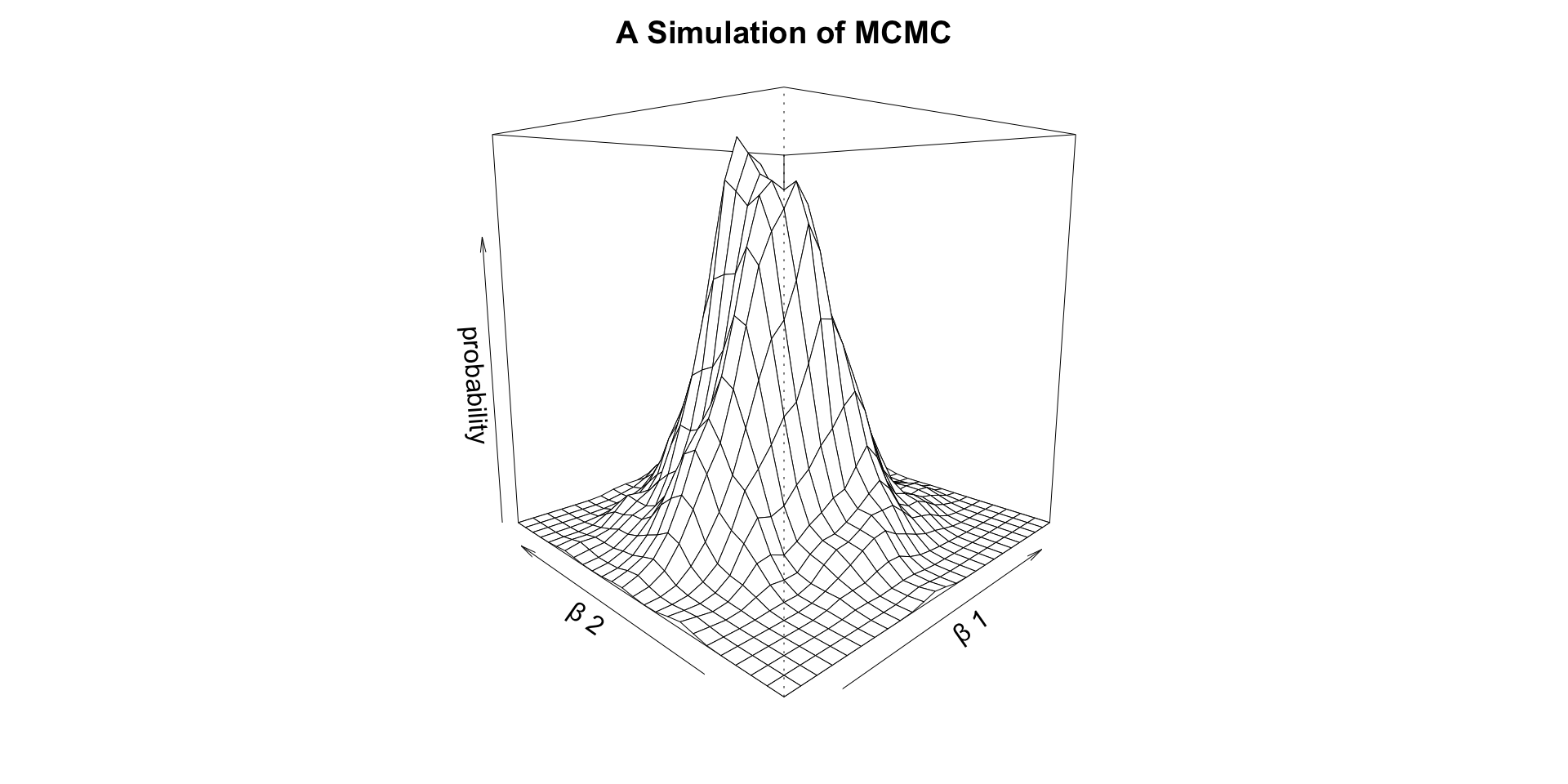
scale reduction factor on split chains (at convergence, Rhat = 1).Markov Chain Monte Carlo (MCMC)
Questions?
Questions?