Data Visualization With Stata (The Basics)

1 Introduction

99% of data visualization work seems to consist of creating bar graphs (graph bar y, over(x)) and scatterplots (twoway scatter y x). (For the sake of completeness, I am also going to mention histograms (histogram x).)

Note: In some commands, I use /// so that Stata commands can be on multiple lines.

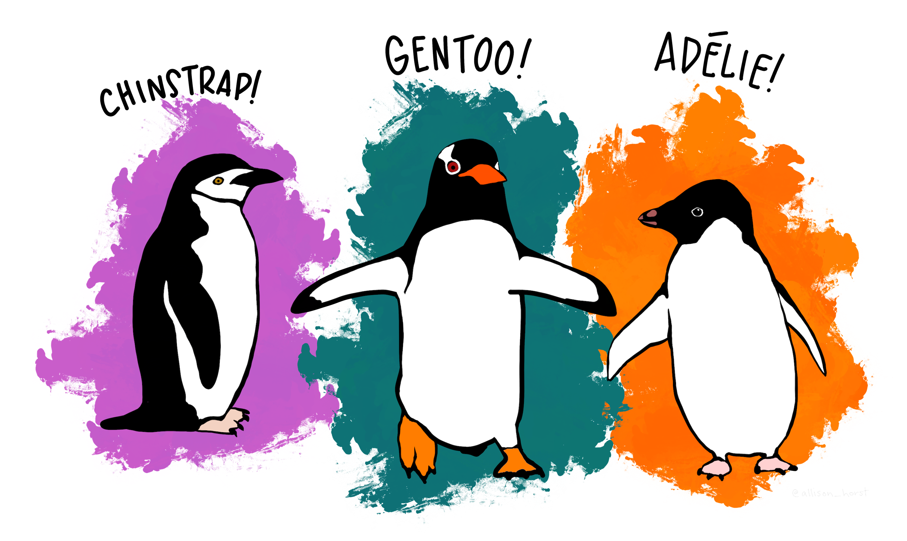
This is a quick guide to these ideas using the Palmer Penguins Data.

2 Setup

clear all

use "penguins.dta", clear

Or, click here to download the data.

I am not a particular fan of the default s2color graph scheme in earlier versions of Stata. In earlier versions of Stata, I might use the s1color scheme by typing set scheme s1color. This handout makes use of the stcolor graph scheme which is the default in newer versions of Stata.

3 Histogram: histogram x

histogram body_mass_g, title("Body Mass of Penguins") xtitle("Body Mass")

histogram

4 Bar Graph: graph bar

4.1 Counting Up Numbers In Each Group: graph bar, over(x)

graph bar, over(species) title("Penguin Species")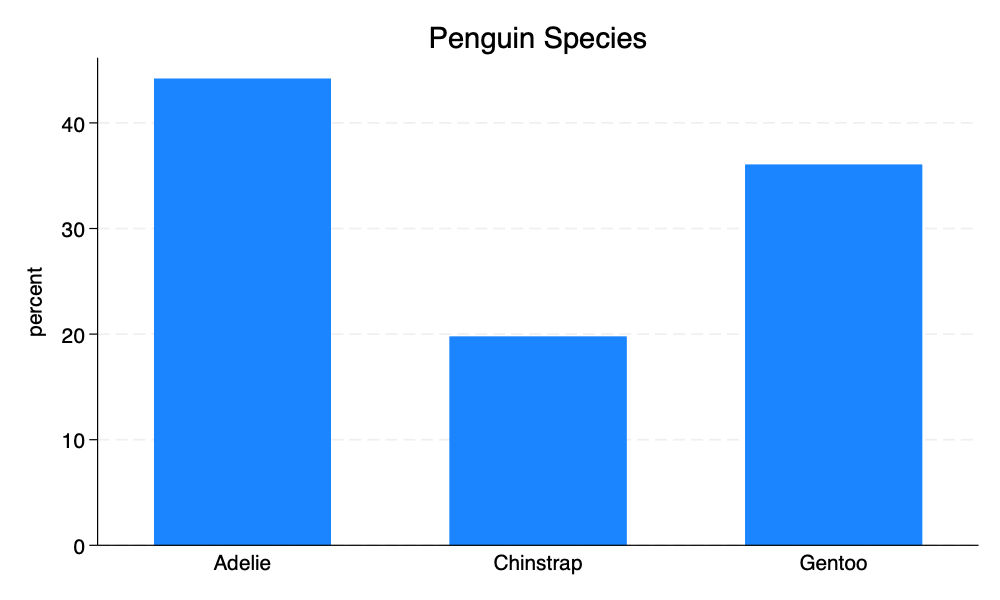

bar graph

4.2 Average Of A Continuous Variable Across Groups: graph bar y, over(x)

graph bar body_mass_g, over(species) title("Body Mass of Penguin Species")

bar graph

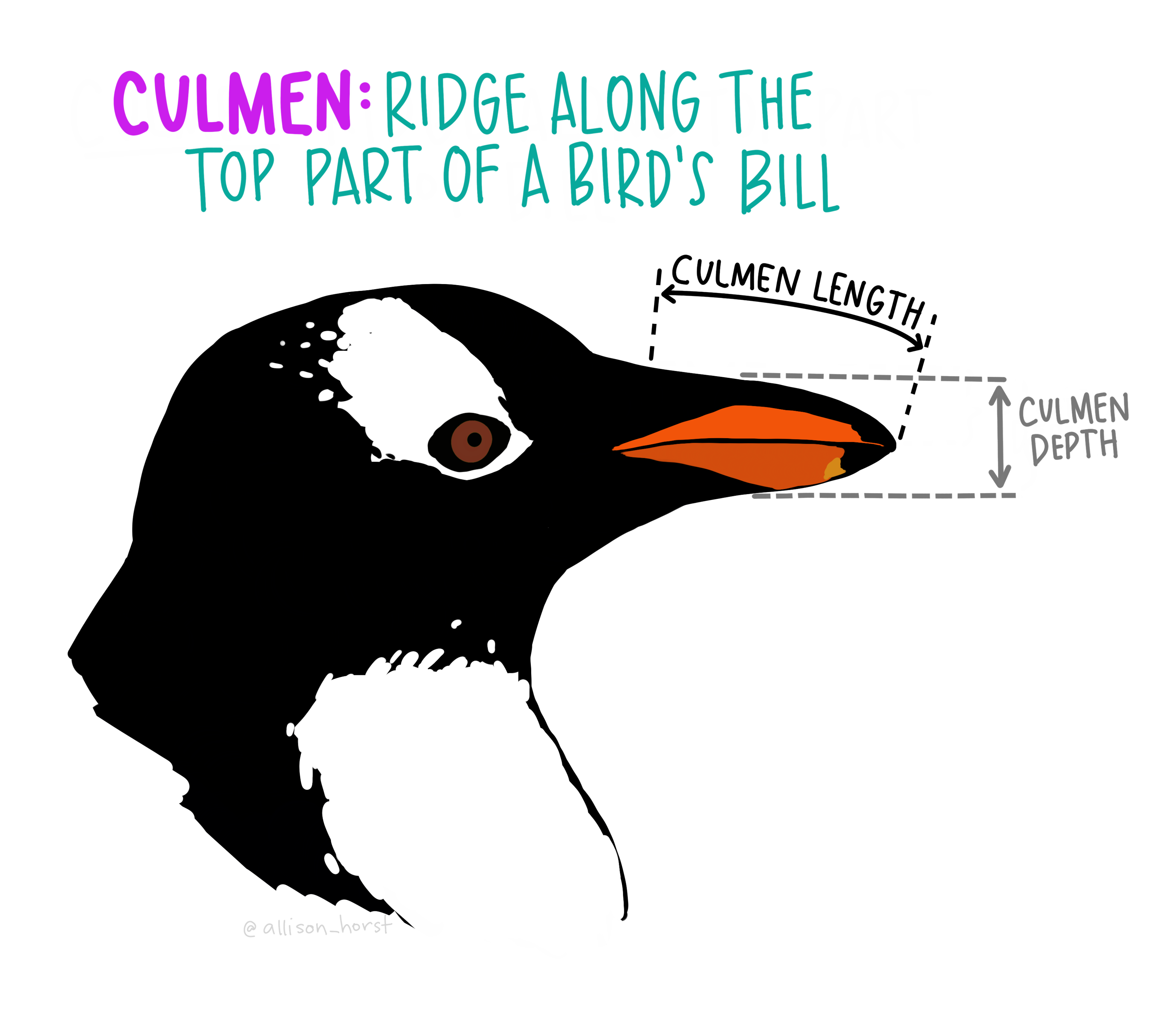
5 Scatterplot: twoway scatter y x

twoway scatter culmen_length_mm body_mass_g, ///
title("Penguin Culmen Length by Body Mass") /// 
xtitle("Body Mass") ///
ytitle("Culmen Length")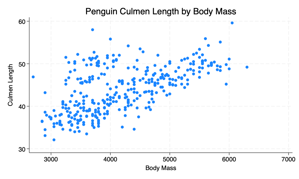

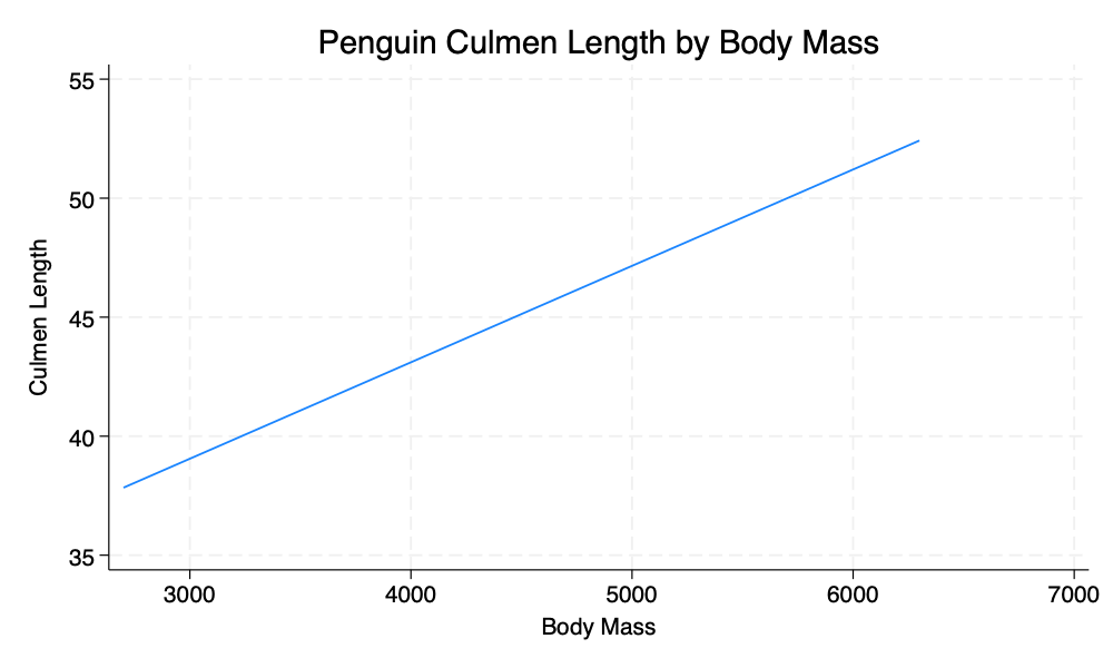
scatterplot

6 Linear Fit: twoway lfit y x

twoway lfit culmen_length_mm body_mass_g, ///
title("Penguin Culmen Length by Body Mass") /// 
xtitle("Body Mass") ///
ytitle("Culmen Length")

scatterplot

histogram bar graph bar graph scatterplot scatterplot