Bayesian and Frequentist Multilevel Modeling
1 Introduction
\[y_{ij} = \beta_0 + \beta_1 x_{1i} + u_{0j} + u_{1j} x + e_{ij}\]
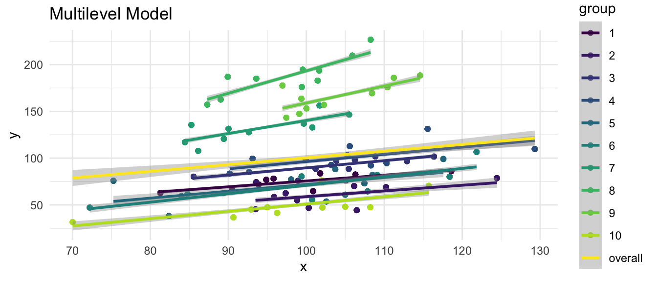
All multilevel models account for group structure, in estimating the association of \(x\) and \(y\), by including a random intercept (\(u_0\)), and possibly one or more random slope terms (\(u_1, u_2, etc....\)).
Bayesian models may offer some advantages over frequentist models, but may be substantially slower to converge.
2 Conceptual Appropriateness
Following Kruschke (2014) all Bayesian models have a conceptual appropriateness.
In frequentist reasoning we are estimating the probability of observing data at least as extreme as our data, while assuming a null hypothesis (\(H_0\)). As has been noted, \(H_0\), e.g. \(\beta = 0\), or \(\bar{x}_A - \bar{x}_B = 0\), is very often not a substantively interesting or substantively meaningful hypothesis.
In Bayesian analysis, we are not rejecting a null hypothesis. Instead, we are directly estimating the value of a parameter such as \(\beta\) and are indeed estimating a full probability distribution for this parameter.
3 Accepting the Null Hypothesis (\(H_0\))
The Bayesian approach means that we have the ability to accept the null hypothesis \(H_0\) (Kruschke & Liddell, 2018). This ability to accept \(H_0\) might possibly lead to theory simplification (Gallistel, 2009; Morey et al., 2018), as well as to a lower likelihood of the publication bias that results from frequentist methods predicated upon the rejection of \(H_0\) (Kruschke & Liddell, 2018).
4 Model Comparison
Relatedly, Bayesian approaches allow one to compare an alternative model \(H_A\) with a null model \(H_0\), or to simply compare two alternative statistical models (\(H_1\) vs. \(H_2\)). Bayesian models may have a better perspective on these kinds of statistical comparisons than do frequentist approaches. As Jarosz et al. (2014) note:
“All Bayesian approaches are comparisons of models. This means that a Bayes factor considers the likelihood of both the null and the alternative hypothesis. From the researcher’s standpoint, this is likely closer to their overall goal than simply rejecting the null hypothesis.”
5 Prior Information
Bayesian models allow one to incorporate prior information about a parameter of interest.
Prior information may come from the prior research literature, e.g. from systematic reviews or meta-analyses, or expert opinion or clinical wisdom.
Kruschke (2014) points out that “No analysis is immune to false alarms, because randomly sampled data will occasionally contain accidental coincidences of outlying values.” However, according to Kruschke (2014) careful use of priors may reduce the probability of false alarms.
6 Multiple Comparisons
As Kruschke (2014) observes, multiple comparisons (especially when they are post hoc) are less of a concern for Bayesian analysis than they are for a frequentist analysis:
“In a Bayesian analysis, however, there is just one posterior distribution over the parameters that describe the conditions. That posterior distribution is unaffected by the intentions of the experimenter, and the posterior distribution can be examined from multiple perspectives however is suggested by insight and curiosity.”
7 Smaller Samples
Bayesian multilevel models may be better with small samples (Rognli et al., 2022; van de Schoot et al., 2015), especially samples with small numbers of Level 2 units (Hox et al., 2012). Some of this advantage may occur when parameters are not normally distributed (Muthen & Asparouhov, 2012). It appears that much of this improvement in performance is dependent upon the use of informative priors (Smid et al., 2020), and that Bayesian models with small samples may provide worse estimates than maximum likelihood estimates when less informative, or inaccurate, priors are used (McNeish, 2016).
8 Full Distribution of Parameters
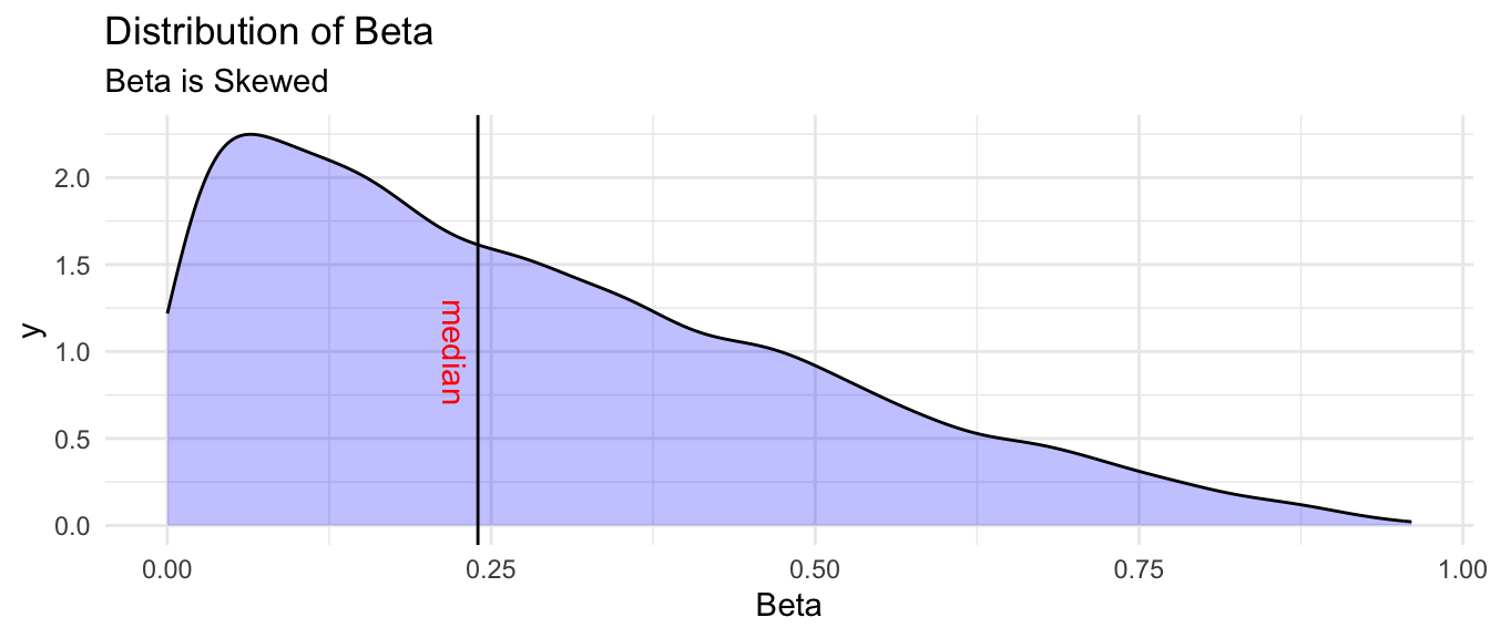
Bayesian models of all kinds provide full distributions of the parameters (e.g. \(\beta\)’s and random effects (\(u\)’s))–both singly and jointly–rather than only point estimates.
Information about the full distribution of a parameter, such as the estimate of the probability distribution of values of a risk factor, a protective factor, or the effect of an intervention, may be substantively meaningful (Rindskopf, 2020). Such information may be especially important when the distribution of a regression parameter is non-normal (Finch & Bolin, 2017; van de Schoot et al., 2014) e.g. in smaller samples.
As Stata Corporation notes, “In a Bayesian multilevel model, random effects are model parameters just like regression coefficients and variance components” (StataCorp, 2020). This ability to estimate the distributions of these random effects means that the distribution of the random effect for one group can be compared to another. For example, the distribution of a parameter in one country could be directly compared to the distribution of that same parameter in another country. One could even estimate the probability that a particular \(\beta\) had a higher value in one group (e.g. country), than in another. As Balov (2016) suggests, this Bayesian approach allows us to “quantify the credibility” of these comparisons, which would not be possible with a frequentist approach. Rognli et al. (2022) make a similar point about estimating the probability of a practically or substantively meaningful effect size.
As an example, Stunnenberg et al. (2018) conducted a Bayesian analysis where the results of the multilevel analysis were used to inform treatment decisions. Here the data were repeated measures on patients, and thus the patients were the groups: “On completion of each treatment set, a Bayesian analysis was conducted to calculate the posterior probability of mexiletine [treatment] producing a clinically meaningful difference in the individual patient.”
9 Distributional Models
Bayesian estimators allow one to directly model \(\sigma_{u_0}\), the variance of the Level 2 units, as a function of covariates (Burkner, 2018). This potentially allows for the opportunity for this variation to become an outcome parameter of substantive interest.
10 Non-Linear Terms
Bayesian estimators allow for the incorporation of non-linear terms (Burkner, 2018). Such non-linear terms offer ways of non-parametrically fitting curvature. An open question is whether such methods represent a kind of over-fitting. A related question is the degree to which non-linear terms provide substantively interpretable results.
11 Maximal Models
Hypothetically, one might imagine that there could be group level unobserved factors which affect many regression slopes–i.e. the relationship between multiple predictors (e.g. \(x_1\), \(x_2\), \(x_3\), etc.) and outcome variable \(y\). Arguably, were one to ignore these unobserved factors in statistical estimation, they would show up either in an error term (\(e_i\) or \(u_0\)), or in the regression coefficients (\(\beta\)). Were they to show up in the regression coefficients this would represent statistical bias and a substantive mis-estimation of important effects. Thus, there is a conceptual argument for including as many random effects—i.e. random slopes—in a statistical model as possible.
Bayesian estimators more readily allow for the estimation of so called maximal models (Barr et al., 2013; Frank, 2018), which allow for the inclusion of a large number of random slopes, e.g. \(u_1, u_2, u_3, ..., etc.\) even when some of those estimated slopes are close to 0.
It should be noted that Matuschek et al. (2017) argue that such a maximal approach may lead to a loss of statistical power and further argue that one should adhere to “a random effect structure that is supported by the data.”
In contrast, Nalborczyk et al. (2019) argue that maximal models are supported under the Bayesian approach. Oberauer (2022) also argues for including multiple random slopes. Schielzeth & Forstmeier (2009) make a similar argument from a frequentist perspective.


