Multiple Methods of Longitudinal Data Analysis

DRAFT Notes

Author

Andy Grogan-Kaylor

Published

December 15, 2023

1 Some Data

Code

clear all

set seed 3846 //  set random seed

quietly set obs 10 // 10 observations

generate id = _n // id number

quietly expand 3 // expand by 3

sort id // sort by id

bysort id: generate t = _n // time variable

generate x = rnormal(10, 3) // random normal variable

generate w = rbinomial(1, .3) // random binomial variable

generate e = rnormal(0, 1) // random error

generate y = x + w + e // regression equation

drop e // drop error

list // list out the data

save longitudinal.dta, replace
     | id   t          x   w          y |
     |----------------------------------|
  1. |  1   1   13.26895   0   11.69778 |
  2. |  1   2   5.669146   1     6.4028 |
  3. |  1   3   11.32535   0   11.00579 |
  4. |  2   1   7.237092   0   6.865333 |
  5. |  2   2   12.60327   1   15.93668 |
     |----------------------------------|
  6. |  2   3   14.30695   1   13.92043 |
  7. |  3   1   6.360627   0   7.093182 |
  8. |  3   2   7.607124   0   7.378952 |
  9. |  3   3   11.15448   0   11.90395 |
 10. |  4   1   7.403773   1   10.07775 |
     |----------------------------------|
 11. |  4   2    11.1741   0   10.86197 |
 12. |  4   3   7.016891   0    5.84125 |
 13. |  5   1   7.085833   0   7.996722 |
 14. |  5   2   8.618052   0   9.414988 |
 15. |  5   3   10.27657   0   10.59132 |
     |----------------------------------|
 16. |  6   1   7.937543   1   10.02182 |
 17. |  6   2   12.00493   0   10.40057 |
 18. |  6   3   11.22594   1   12.66391 |
 19. |  7   1   11.34407   0   10.74489 |
 20. |  7   2   11.35657   0    11.4781 |
     |----------------------------------|
 21. |  7   3    14.3872   0   15.16246 |
 22. |  8   1   11.72829   1   11.94959 |
 23. |  8   2   8.028893   1   8.781265 |
 24. |  8   3   11.90905   1   12.49115 |
 25. |  9   1   9.205235   0   8.002105 |
     |----------------------------------|
 26. |  9   2   5.909642   1     8.8732 |
 27. |  9   3   16.80353   0   16.67801 |
 28. | 10   1   6.183664   0   6.201822 |
 29. | 10   2   7.644044   0    5.58361 |
 30. | 10   3   11.53438   0   11.32048 |
     +----------------------------------+

file longitudinal.dta saved

2 Multilevel Modeling

We assume that \(u_{0i}\) has a normal distribution, but do not directly estimate the values of \(u_{0i}\) for each individual.

\(y_{it} = \beta_0 + \beta_1 x_{it} + \beta_2 w_{it} + u_{0i} + e_{it}\)

Code

use longitudinal.dta, clear

mixed y x i.w || id:
Performing EM optimization Performing gradient-based optimization: 
Iteration 0:  Log likelihood = -41.789697  
Iteration 1:  Log likelihood = -41.654948  
Iteration 2:  Log likelihood = -41.653312  
Iteration 3:  Log likelihood =  -41.65331  

Computing standard errors ...

Mixed-effects ML regression                          Number of obs    =     30
Group variable: id                                   Number of groups =     10
                                                     Obs per group:
                                                                  min =      3
                                                                  avg =    3.0
                                                                  max =      3
                                                     Wald chi2(2)     = 236.62
Log likelihood =  -41.65331                          Prob > chi2      = 0.0000

------------------------------------------------------------------------------
           y | Coefficient  Std. err.      z    P>|z|     [95% conf. interval]
-------------+----------------------------------------------------------------
           x |    .938261   .0626023    14.99   0.000     .8155627    1.060959
         1.w |   1.682743   .3765298     4.47   0.000     .9447577    2.420728
       _cons |   .3540235   .6672312     0.53   0.596    -.9537257    1.661773
------------------------------------------------------------------------------

------------------------------------------------------------------------------
  Random-effects parameters  |   Estimate   Std. err.     [95% conf. interval]
-----------------------------+------------------------------------------------
id: Identity                 |
                  var(_cons) |   1.66e-15   1.53e-11             0           .
-----------------------------+------------------------------------------------
               var(Residual) |   .9408329   .2429279      .5671891     1.56062
------------------------------------------------------------------------------
LR test vs. linear model: chibar2(01) = 1.4e-14       Prob >= chibar2 = 1.0000

3 Fixed Effects

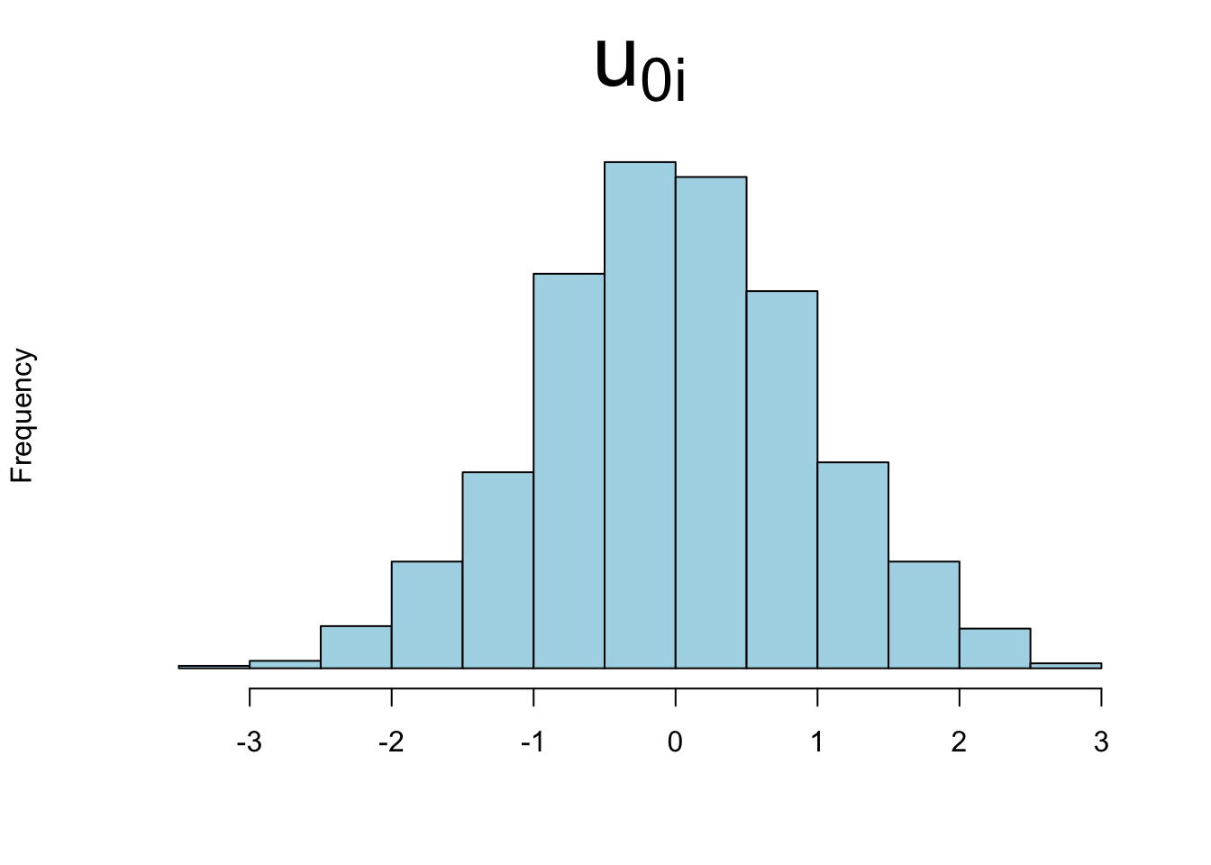
We assume that the \(u_{0i}\) are in fact, estimable. However, we end up estimating \(y_{it} - \bar y_i = \beta_1 (x_{it} - \bar x_i) + \beta_2 (w_{it} - \bar w_i) + (e_{it} - \bar e_i)\). The \(u_{0i}\) have dropped out of this equation.

\(y_{it} = \beta_0 + \beta_1 x_{it} + \beta_2 w_{it} + u_{0i} + e_{it}\)

Code

use longitudinal.dta, clear

xtreg y x i.w, i(id) fe
Fixed-effects (within) regression               Number of obs     =         30
Group variable: id                              Number of groups  =         10

R-squared:                                      Obs per group:
     Within  = 0.9142                                         min =          3
     Between = 0.8102                                         avg =        3.0
     Overall = 0.8673                                         max =          3

                                                F(2, 18)          =      95.93
corr(u_i, Xb) = -0.3779                         Prob > F          =     0.0000

------------------------------------------------------------------------------
           y | Coefficient  Std. err.      t    P>|t|     [95% conf. interval]
-------------+----------------------------------------------------------------
           x |    .987199   .0714222    13.82   0.000     .8371465    1.137252
         1.w |   2.757344   .5380926     5.12   0.000     1.626853    3.887834
       _cons |  -.4908022   .8026548    -0.61   0.549    -2.177117    1.195513
-------------+----------------------------------------------------------------
     sigma_u |  .87126686
     sigma_e |  .93451278
         rho |  .46501875   (fraction of variance due to u_i)
------------------------------------------------------------------------------
F test that all u_i=0: F(9, 18) = 1.59                       Prob > F = 0.1919

4 Difference in Differences

???

5 Cross Lagged Regression

Similar to before, there is an equation predicting y.

\(y_{2i} = \beta_0 + \beta_1 y_{1i} + \beta_2 x_{1i} + \beta_3 w_{2i} + e_i\)

However, we need an equation for each time point, so:

\(y_{3i} = \beta_0 + \beta_1 y_{2i} + \beta_2 x_{2i} + \beta_3 w_{2i} + e_i\)

And, there are also equations predicting x.

\(x_{2i} = \beta_0 + \beta_1 x_{1i} + \beta_2 y_{1i} + \beta_3 w_{1i} + e_i\)

\(x_{3i} = \beta_0 + \beta_1 x_{2i} + \beta_2 y_{2i} + \beta_3 w_{2i} + e_i\)

In cross-lagged regression, we need the data to be in wide format rather than long format.

Code

use longitudinal.dta, clear

reshape wide y x w, i(id) j(t) // reshape data to wide

save longitudinalWIDE.dta, replace
(j = 1 2 3)

Data                               Long   ->   Wide
-----------------------------------------------------------------------------
Number of observations               30   ->   10          
Number of variables                   5   ->   10          
j variable (3 values)                 t   ->   (dropped)
xij variables:
                                      y   ->   y1 y2 y3
                                      x   ->   x1 x2 x3
                                      w   ->   w1 w2 w3
-----------------------------------------------------------------------------

file longitudinalWIDE.dta saved
Code

use longitudinalWIDE.dta, clear

sem (y2 <- y1 x1 w1) ///
(x2 <- x1 y1 w1) ///
(y3 <- y2 x2 w2) ///
(x3 <- x2 y2 w2)  
Endogenous variables
  Observed: y2 x2 y3 x3

Exogenous variables
  Observed: y1 x1 w1 w2

Fitting target model:
Iteration 0:  Log likelihood = -126.89265  
Iteration 1:  Log likelihood = -126.89265  

Structural equation model                                   Number of obs = 10
Estimation method: ml

Log likelihood = -126.89265

------------------------------------------------------------------------------
             |                 OIM
             | Coefficient  std. err.      z    P>|z|     [95% conf. interval]
-------------+----------------------------------------------------------------
Structural   |
  y2         |
          y1 |    -.06638   1.722865    -0.04   0.969    -3.443134    3.310374
          x1 |  -.1142004    1.22043    -0.09   0.925    -2.506199    2.277798
          w1 |   .9129669   4.046881     0.23   0.822    -7.018773    8.844707
       _cons |   10.84123    5.48777     1.98   0.048     .0853985    21.59706
  -----------+----------------------------------------------------------------
  x2         |
          y1 |   1.077149   1.270605     0.85   0.397    -1.413191    3.567489
          x1 |  -1.050991   .9000609    -1.17   0.243    -2.815078    .7130958
          w1 |  -.2019809   2.984554    -0.07   0.946      -6.0516    5.647638
       _cons |   8.580689   4.047204     2.12   0.034     .6483162    16.51306
  -----------+----------------------------------------------------------------
  y3         |
          y2 |   .6385229   .7520661     0.85   0.396    -.8354996    2.112545
          x2 |  -.6869322   .9228791    -0.74   0.457    -2.495742    1.121878
          w2 |   .6030497   2.657096     0.23   0.820    -4.604762    5.810862
       _cons |   12.06822   3.779402     3.19   0.001     4.660724    19.47571
  -----------+----------------------------------------------------------------
  x3         |
          y2 |   .7641998   .6168695     1.24   0.215    -.4448422    1.973242
          x2 |  -.8415779    .756976    -1.11   0.266    -2.325223    .6420677
          w2 |   .6179903   2.179438     0.28   0.777     -3.65363     4.88961
       _cons |   12.10439   3.099991     3.90   0.000     6.028522    18.18026
-------------+----------------------------------------------------------------
    var(e.y2)|   7.584673   3.391969                      3.156952    18.22241
    var(e.x2)|   4.125296   1.844888                      1.717063    9.911148
    var(e.y3)|   6.049814   2.705559                      2.518101    14.53486
    var(e.x3)|   4.070208   1.820252                      1.694134    9.778798
------------------------------------------------------------------------------
LR test of model vs. saturated: chi2(10) = 85.21          Prob > chi2 = 0.0000

6 Summary 1

Code
Method <- c("Multilevel Modeling",
            "Fixed Effects",
            "Cross Lagged Regression")

`Control for Time Invariant Observed` <- c("yes",
                                           "yes",
                                           "yes")

`Control for Time Varying Observed` <- c("yes",
                                         "yes",
                                         "yes")

`Control for Time Invariant Unobserved` <- c("partially",
                                             "yes",
                                             "no")

`Control for Time Varying Unobserved` <- c("no",
                                           "no",
                                           "no")
`Estimate Reciprocal Causality` <- c("no",
                                     "no",
                                     "yes")

`Control for Earlier or Baseline y` <- c("automatic",
                                         "automatic",
                                         "must explicitly specify")

mytable <- data.frame(Method,
                      `Control for Time Invariant Observed`,
                      `Control for Time Varying Observed`,
                      `Control for Time Invariant Unobserved`,
                      `Control for Time Varying Unobserved`,
                      `Estimate Reciprocal Causality`,
                      `Control for Earlier or Baseline y`,
                      check.names = FALSE)

pander:: pander(mytable)
Table continues below
Method Control for Time Invariant Observed
Multilevel Modeling yes
Fixed Effects yes
Cross Lagged Regression yes
Table continues below
Control for Time Varying Observed Control for Time Invariant Unobserved
yes partially
yes yes
yes no
Table continues below
Control for Time Varying Unobserved Estimate Reciprocal Causality
no no
no no
no yes
Control for Earlier or Baseline y
automatic
automatic
must explicitly specify

Footnotes

  1. Some of the decisions in this table are arguable.↩︎