1 Mar 2023
This example uses data from https://stats.idre.ucla.edu/stata/examples/mlm-imm/introduction-to-multilevel-modeling-by-kreft-and-de-leeuwchapter-4-analyses/
. use https://stats.idre.ucla.edu/stat/examples/imm/imm23, clear
. label variable ses "Socioeconomic Status" // correct spelling of variable label
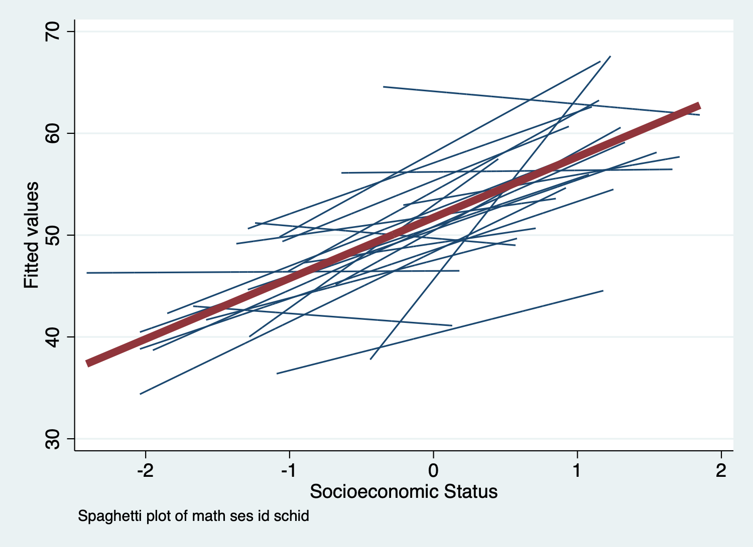
. spagplot math ses, id(schid)
. graph export graph1.png, width(1500) replace
file /Users/agrogan/Desktop/GitHub/multilevel/spaghetti-plot/Stata/graph1.png saved as
    PNG format
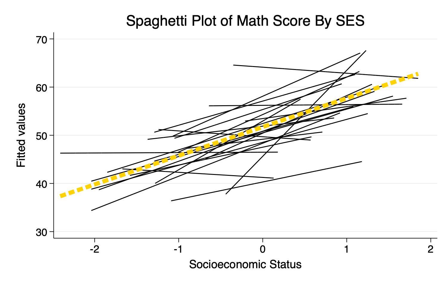
Schemes are very helpful in making better looking Stata graphs. A useful Stata scheme is
s1color. Useful user written schemes arelean2,plottig(typefindit lean2orfindit plottigto install these), and my own Michigan Stata graph scheme.
. spagplot math ses, id(schid) ///
> scheme(michigan) ///
> title("Spaghetti Plot of Math Score By SES") ///
> note(" ") // blank "note" since title explains this graph
. graph export graph2.png, width(1500) replace
file /Users/agrogan/Desktop/GitHub/multilevel/spaghetti-plot/Stata/graph2.png saved as
    PNG format
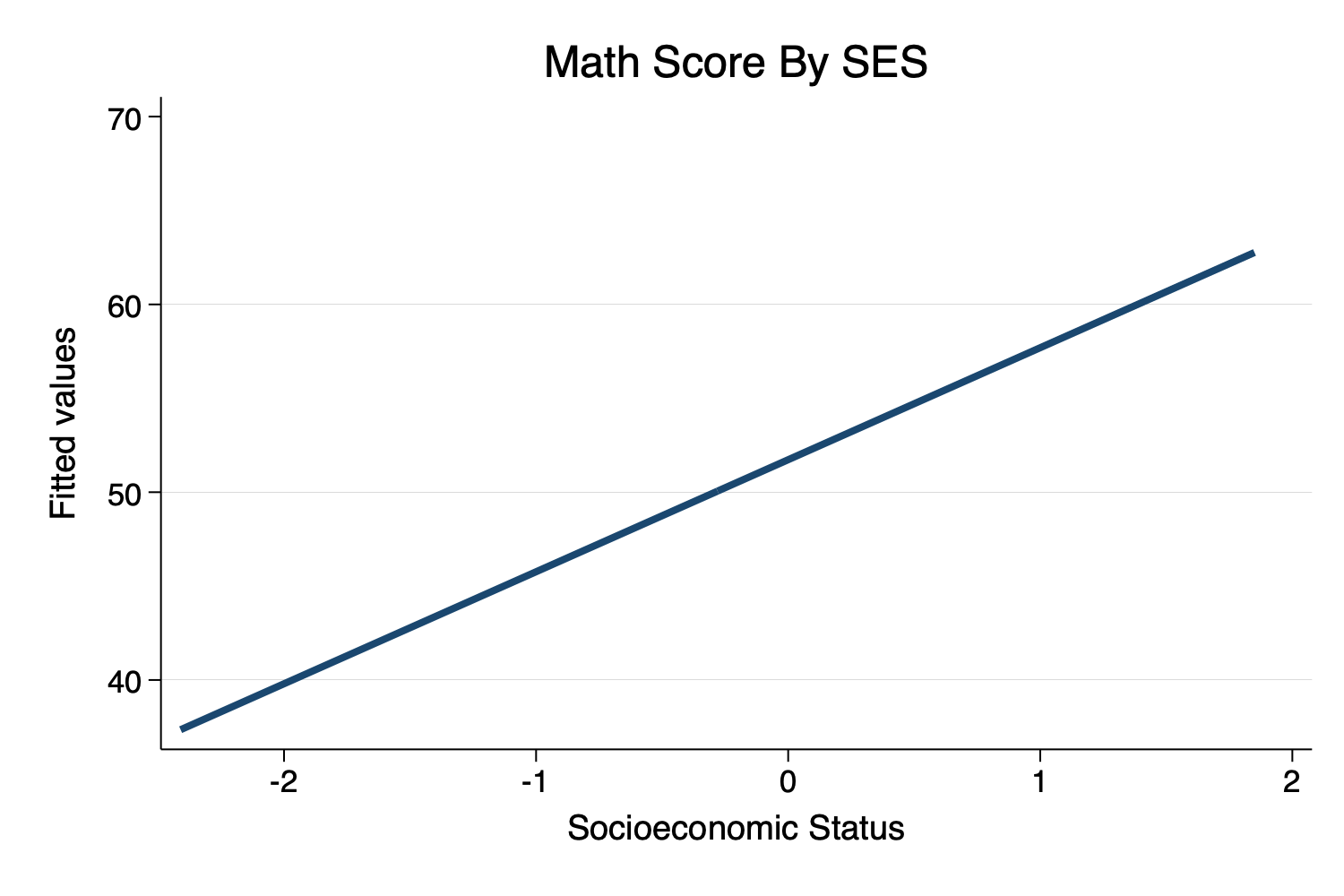
twoway Syntax. twoway lfit math ses, scheme(michigan) title("Math Score By SES")
. graph export graph3.png, width(1500) replace
file /Users/agrogan/Desktop/GitHub/multilevel/spaghetti-plot/Stata/graph3.png saved as
    PNG format
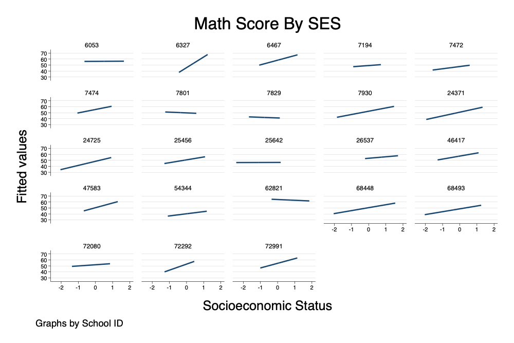
This ONLY works well with a limited number of schools.
. twoway lfit math ses, scheme(michigan) by(schid, title("Math Score By SES"))
. graph export graph4.png, width(1000) replace
file /Users/agrogan/Desktop/GitHub/multilevel/spaghetti-plot/Stata/graph4.png saved as
    PNG format
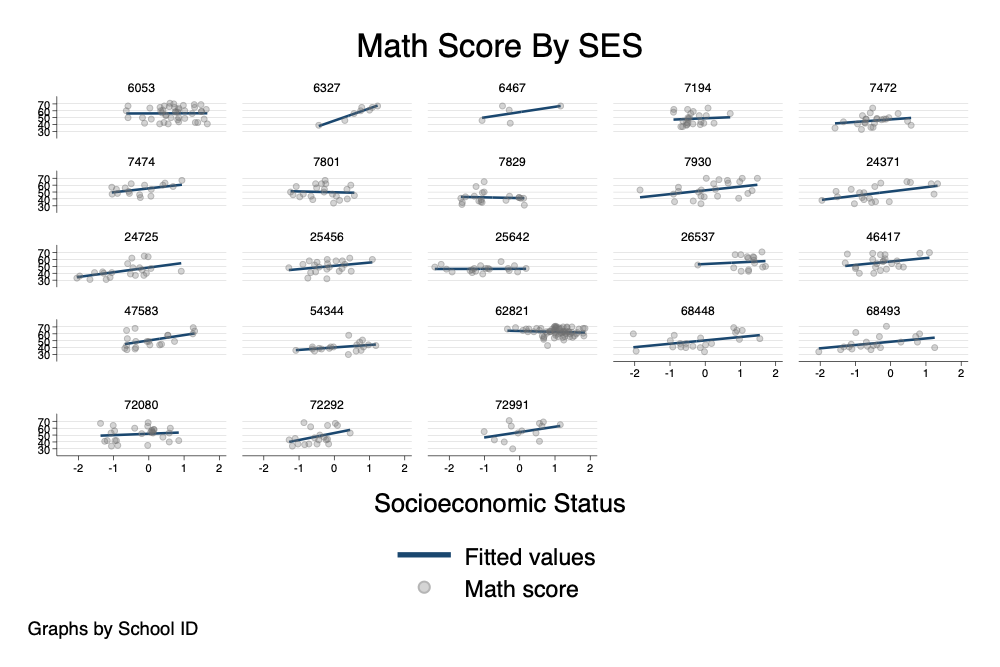
. twoway (lfit math ses) ///
> (scatter math ses, mcolor(gs7%30)), /// color gs7 @ 30% transparency
> scheme(michigan) by(schid, title("Math Score By SES"))
. graph export graph5.png, width(1000) replace
file /Users/agrogan/Desktop/GitHub/multilevel/spaghetti-plot/Stata/graph5.png saved as
    PNG format
A sometimes unacknowledged point is that spaghetti plots–unless we take steps to correct this–reflect unadjusted, or bivariate associations.
We may sometimes wish to develop a spaghetti plot that reflects the adjusted estimates from our models.
To do this we first estimate a multilevel model.
. mixed math ses meanses || schid: // multilevel model; random intercept; no random effect
> s

Performing EM optimization:

Performing gradient-based optimization:

Iteration 0:   log likelihood = -1871.9169
Iteration 1:   log likelihood = -1871.9169

Computing standard errors:

Mixed-effects ML regression                     Number of obs     =        519
Group variable: schid                           Number of groups  =         23
                                                Obs per group:
                                                              min =          5
                                                              avg =       22.6
                                                              max =         67
                                                Wald chi2(2)      =      69.58
Log likelihood = -1871.9169                     Prob > chi2       =     0.0000

─────────────┬────────────────────────────────────────────────────────────────
        math │ Coefficient  Std. err.      z    P>|z|     [95% conf. interval]
─────────────┼────────────────────────────────────────────────────────────────
         ses │    3.88476   .6096853     6.37   0.000     2.689799    5.079722
     meanses │   3.281962   1.464135     2.24   0.025     .4123106    6.151614
       _cons │   51.48904   .7582764    67.90   0.000     50.00284    52.97523
─────────────┴────────────────────────────────────────────────────────────────

─────────────────────────────┬────────────────────────────────────────────────
  Random-effects parameters  │   Estimate   Std. err.     [95% conf. interval]
─────────────────────────────┼────────────────────────────────────────────────
schid: Identity              │
                  var(_cons) │   8.931927   3.813085      3.868681    20.62184
─────────────────────────────┼────────────────────────────────────────────────
               var(Residual) │   75.21885   4.778177      66.41333    85.19187
─────────────────────────────┴────────────────────────────────────────────────
LR test vs. linear model: chibar2(01) = 25.58         Prob >= chibar2 = 0.0000
NB that this is a model with only a random intercept, \(u_0\) and no random slopes e.g. \(u_1\), etc….
. predict yhat
(option xb assumed)
. spagplot yhat ses, id(schid) scheme(michigan)
. graph export graph6A.png, width(1500) replace
file /Users/agrogan/Desktop/GitHub/multilevel/spaghetti-plot/Stata/graph6A.png saved as
    PNG format
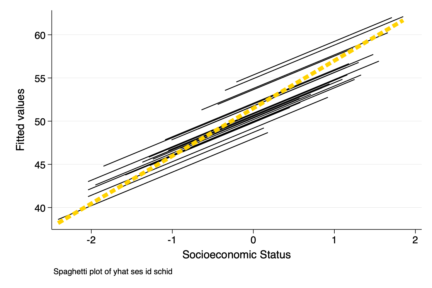
The spaghetti plots so far give an indication of different slopes per school. Below we outline a procedure for (a) developing a spaghetti plot of adjusted estimates; and (b) ensuring that the plot reflects the exact structure of the model e.g. random intercept only, or random intercept + random slope(s).
To carry out this procedure we employ the _b notation in
Stata. For example, _b[_cons] indicates the intercept of
the model while _b[ses] indicates the slope attached to
ses.
We need to carry out a few preliminary calculations.
predict) the random effect(s).summarize) of variables that
we are going to hold constant._b notation
(generate yhat = ...).twoway connect).. mixed math ses meanses || schid: // multilevel model; random intercept; no random effect
> s
Performing EM optimization:
Performing gradient-based optimization:
Iteration 0: log likelihood = -1871.9169
Iteration 1: log likelihood = -1871.9169
Computing standard errors:
Mixed-effects ML regression Number of obs = 519
Group variable: schid Number of groups = 23
Obs per group:
min = 5
avg = 22.6
max = 67
Wald chi2(2) = 69.58
Log likelihood = -1871.9169 Prob > chi2 = 0.0000
─────────────┬────────────────────────────────────────────────────────────────
math │ Coefficient Std. err. z P>|z| [95% conf. interval]
─────────────┼────────────────────────────────────────────────────────────────
ses │ 3.88476 .6096853 6.37 0.000 2.689799 5.079722
meanses │ 3.281962 1.464135 2.24 0.025 .4123106 6.151614
_cons │ 51.48904 .7582764 67.90 0.000 50.00284 52.97523
─────────────┴────────────────────────────────────────────────────────────────
─────────────────────────────┬────────────────────────────────────────────────
Random-effects parameters │ Estimate Std. err. [95% conf. interval]
─────────────────────────────┼────────────────────────────────────────────────
schid: Identity │
var(_cons) │ 8.931927 3.813085 3.868681 20.62184
─────────────────────────────┼────────────────────────────────────────────────
var(Residual) │ 75.21885 4.778177 66.41333 85.19187
─────────────────────────────┴────────────────────────────────────────────────
LR test vs. linear model: chibar2(01) = 25.58 Prob >= chibar2 = 0.0000
. predict u0, reffects
. summarize meanses

    Variable │        Obs        Mean    Std. dev.       Min        Max
─────────────┼─────────────────────────────────────────────────────────
     meanses │        519   -.0012717    .6206429    -1.0685    1.17625
The mean of meanses is -0.00127.
We are using \(\beta_0\), the random
intercept \(u_0\), \(\beta_{ses}\) multiplied by the actual
value of ses, and \(\beta_{meanses}\) multiplied by the mean of
meanses.
. generate yhat2 = _b[_cons] + u0 + _b[ses] * ses + _b[ses] * -.0012717
. twoway scatter yhat2 ses, scheme(michigan)
. graph export graph6B.png, width(1500) replace
file /Users/agrogan/Desktop/GitHub/multilevel/spaghetti-plot/Stata/graph6B.png saved as
    PNG format
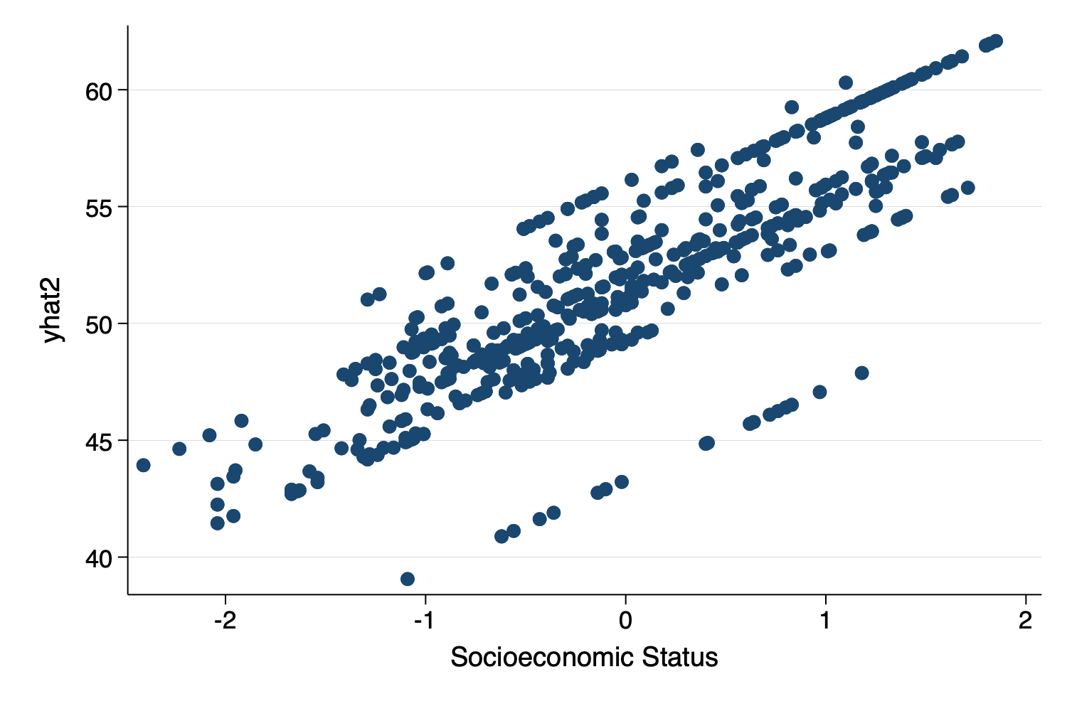
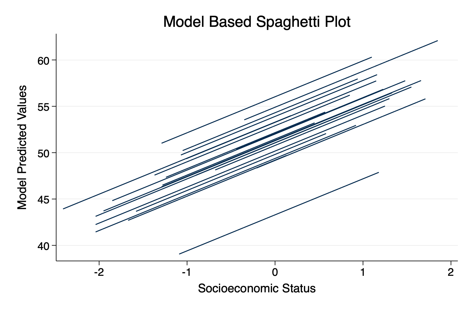
We still have a small amount of work to do to make this look more “spaghetti plot like”.
We are going to use twoway connect to create connected
line plots. We employ option c(L) to ensure that only
ascending values are connected: i.e. each Level 2 unit has their own
regression line. For c(L) to work properly we are going to
need to sort the data by school and ses. Lastly, we’re
going to change the msymbol so that we do not see dots, but
only lines.
. sort schid ses // sort on Level 2 units and x values
. twoway connect yhat2 ses, ///
> lcolor("0 39 76") /// Michigan blue for connecting lines
> title("Model Based Spaghetti Plot") /// title
> xtitle("Socioeconomic Status") /// title for x axis
> ytitle("Model Predicted Values") /// title for y axis
> c(L) /// connect only ascending values
> msymbol(none) /// no marker symbol; only lines
> scheme(michigan) // michigan scheme
. graph export graph7.png, width(1500) replace
file /Users/agrogan/Desktop/GitHub/multilevel/spaghetti-plot/Stata/graph7.png saved as
    PNG format