Scatterplots (twoway scatter y x)
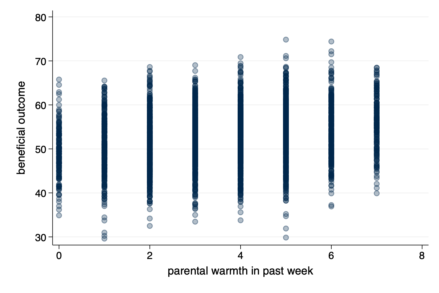
Figure 1: Scatterplot
twoway scatter y x)
Figure 1: Scatterplot
twoway lfit y x)
Figure 2: Linear Fit
twoway lfitci y x)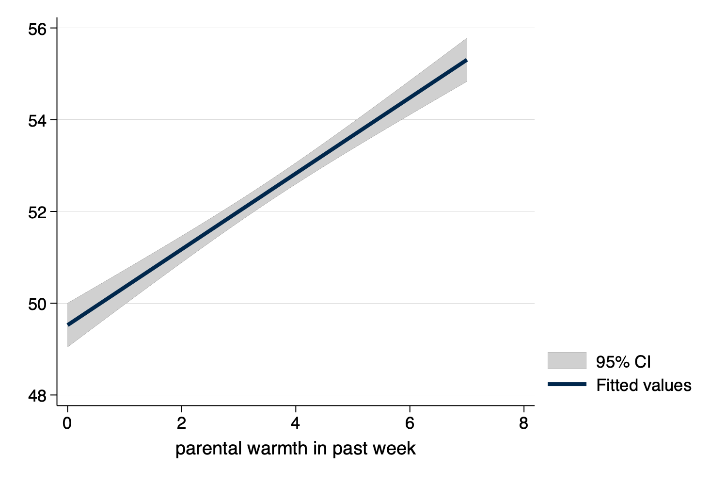
Figure 3: Linear Fit With Confidence Interval
twoway (scatter y x) (lfit y x))twoway (scatter outcome warmth, mcolor(%30)) (lfit outcome warmth)
graph export myscatterlinear.png, width(1500) replace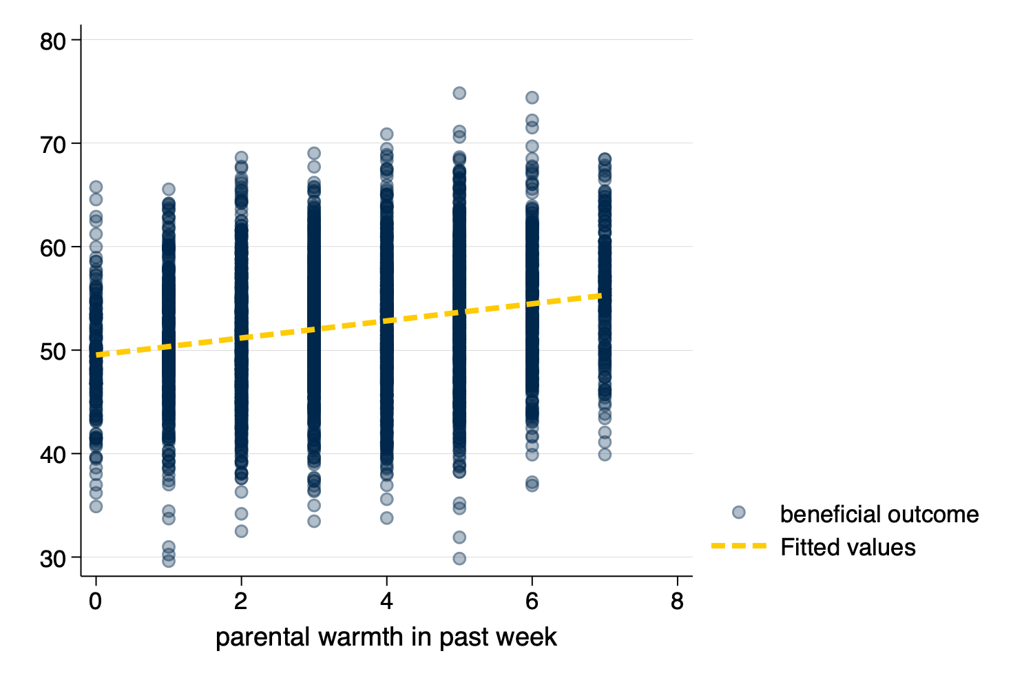
Figure 4: Scatterplot and Linear Fit
spagplot y x, id(group))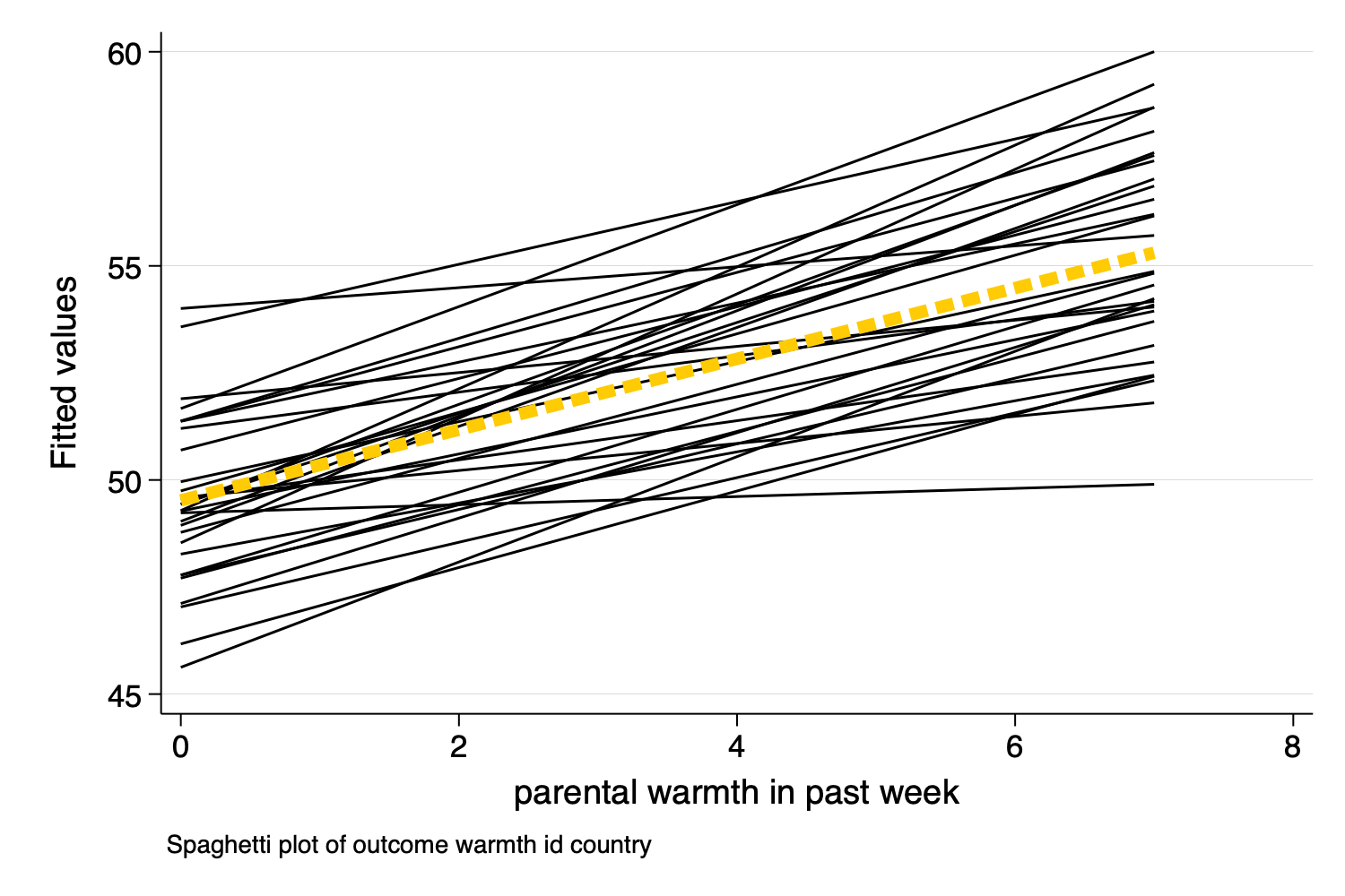
Figure 5: Spaghetti Plot
twoway y x, by(group))Small Multiples, showing a separate graph for each group in
the data, are an increasingly popular data visualization technique.
Below, I build a small multiples graph using the by option
in Stata. I use the aspect option to adjust the aspect
ratio of the graph for better visual presentation.
twoway (scatter outcome warmth, mcolor(%30)) ///
(lfit outcome warmth), ///
by(country) aspect(1)

graph export mysmallmultiples.png, width(1500) replace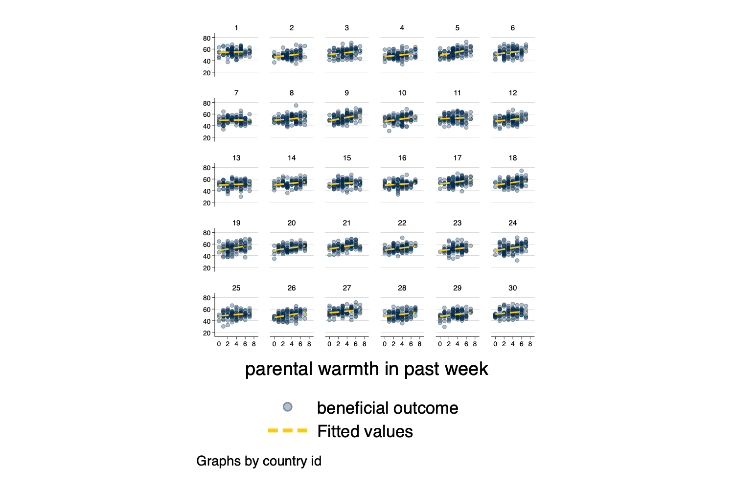
Figure 6: Small Multiples
At times, we may have too many Level 2 units to effectively
display them on a spaghetti plot, or using small
multiples. If this is the case, we may need to randomly
sample Level 2 units. This can be difficult to
accomplish as our standard sample command operates on each
row, or on Level 1 units.
We can accomplish random sampling at Level 2, with a little bit of code.
set seed 3846 // random seed for reproducibility

gen randomid = runiform() // generate a random id variable

* by country (i.e. by Level 2 unit) replace the randomid
* with the first randomid for that country (Level 2 unit)
* so that every person in that country has the same random id

bysort country: replace randomid = randomid[1]

summarize randomid // descriptive statistics for random id

twoway (scatter outcome warmth, mcolor(%30)) /// scatterplot
(lfit outcome warmth) /// linear fit
if randomid < .5, /// only use a subset of randomids
by(country) aspect(1) // by country

quietly: graph export mysmallmultiples2.png, width(1500) replace
(2,970 real changes made)
Variable | Obs Mean Std. dev. Min Max
-------------+---------------------------------------------------------
randomid | 3,000 .6174022 .2374704 .0733026 .9657055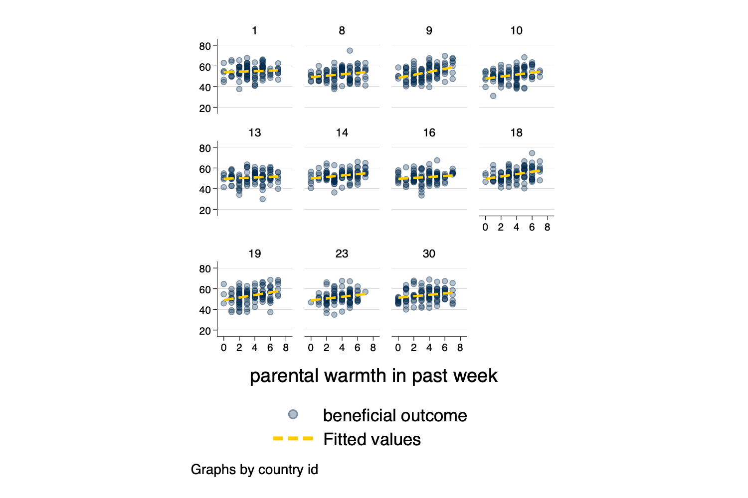
Figure 7: Small Multiples With A Random Sample Of Countries
predict)predict generates a predicted value for every
observation in the data.
[!CAUTION]
Prediction Requires Careful Thinking
In multilevel models, prediction is a complex question. Prediction may–or may not–incorporate the information from the random effects. The procedures below outline graphs that incorporate predictions using the random effects, by using the
predict ..., fittedsyntax.
Performing EM optimization ...

Performing gradient-based optimization:
Iteration 0:  Log likelihood = -9628.1621
Iteration 1:  Log likelihood = -9628.1621

Computing standard errors ...

Mixed-effects ML regression                          Number of obs    =  3,000
Group variable: country                              Number of groups =     30
                                                     Obs per group:
                                                                  min =    100
                                                                  avg =  100.0
                                                                  max =    100
                                                     Wald chi2(3)     = 370.90
Log likelihood = -9628.1621                          Prob > chi2      = 0.0000

------------------------------------------------------------------------------------
           outcome | Coefficient  Std. err.      z    P>|z|     [95% conf. interval]
-------------------+----------------------------------------------------------------
            warmth |   .8330937   .0574809    14.49   0.000     .7204332    .9457543
physical_punishm~t |  -.9937819   .0798493   -12.45   0.000    -1.150284   -.8372801
    1.intervention |   .6406043   .2175496     2.94   0.003      .214215    1.066994
             _cons |   51.65238   .4664841   110.73   0.000     50.73809    52.56668
------------------------------------------------------------------------------------

------------------------------------------------------------------------------
  Random-effects parameters  |   Estimate   Std. err.     [95% conf. interval]
-----------------------------+------------------------------------------------
country: Identity            |
                  var(_cons) |   3.371762   .9613269      1.928279    5.895816
-----------------------------+------------------------------------------------
               var(Residual) |    35.0675    .910002      33.32853    36.89721
------------------------------------------------------------------------------
LR test vs. linear model: chibar2(01) = 204.14 Prob >= chibar2 = 0.0000twoway
Syntaxtwoway (scatter outcome_hat warmth, mcolor(%30)) (lfit outcome_hat warmth)
graph export mypredictedvalues.png, width(1500) replace
twoway (lfit outcome_hat warmth)
graph export mypredictedvalues2.png, width(1500) replace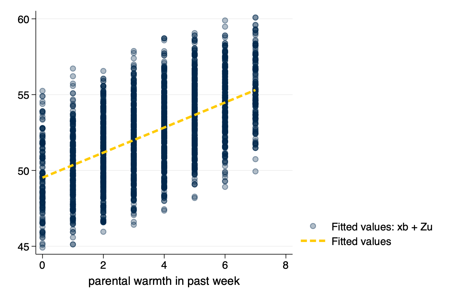
Figure 8: Predicted Values From predict
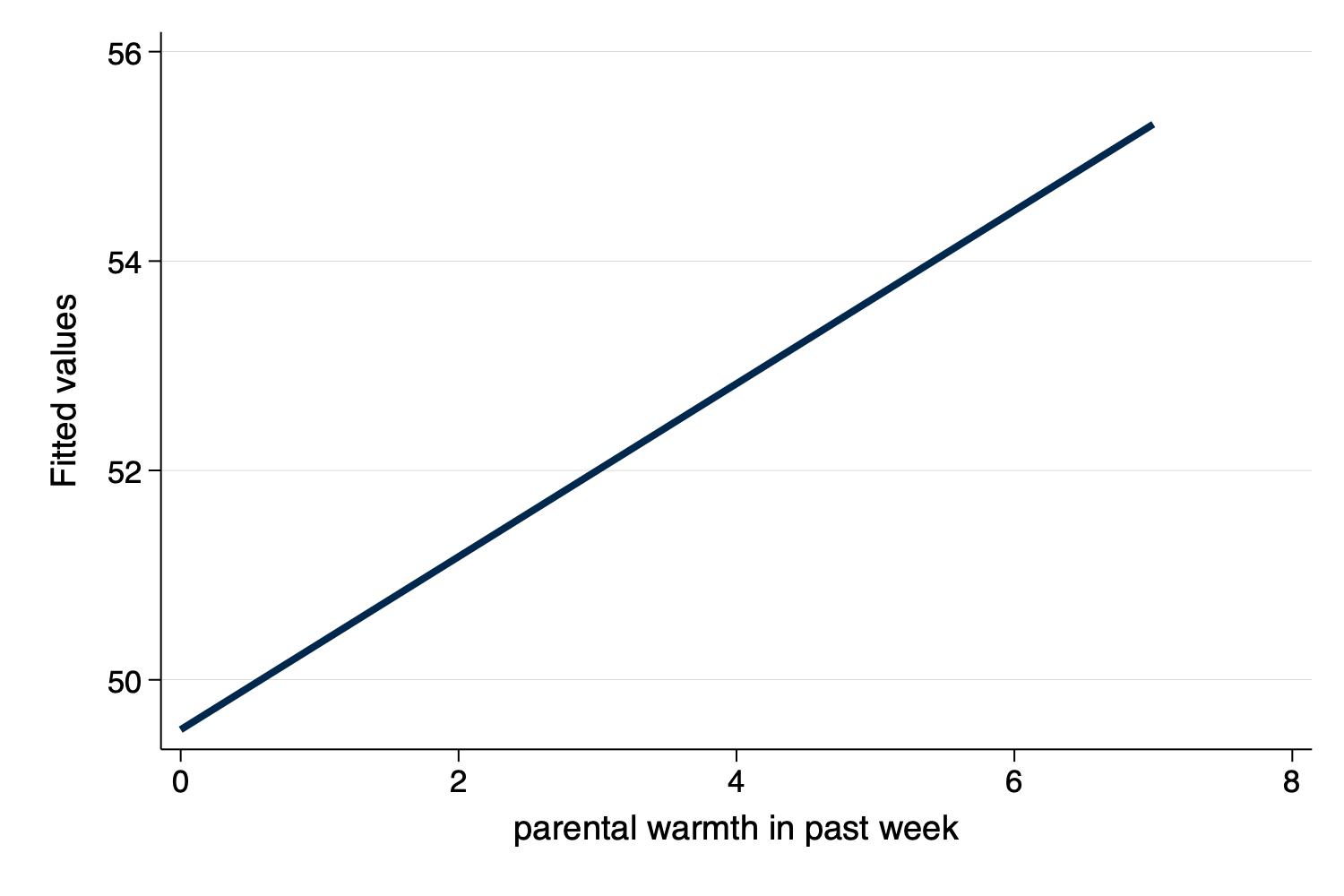
Figure 9: Predicted Values From predict With Only Linear
Fit
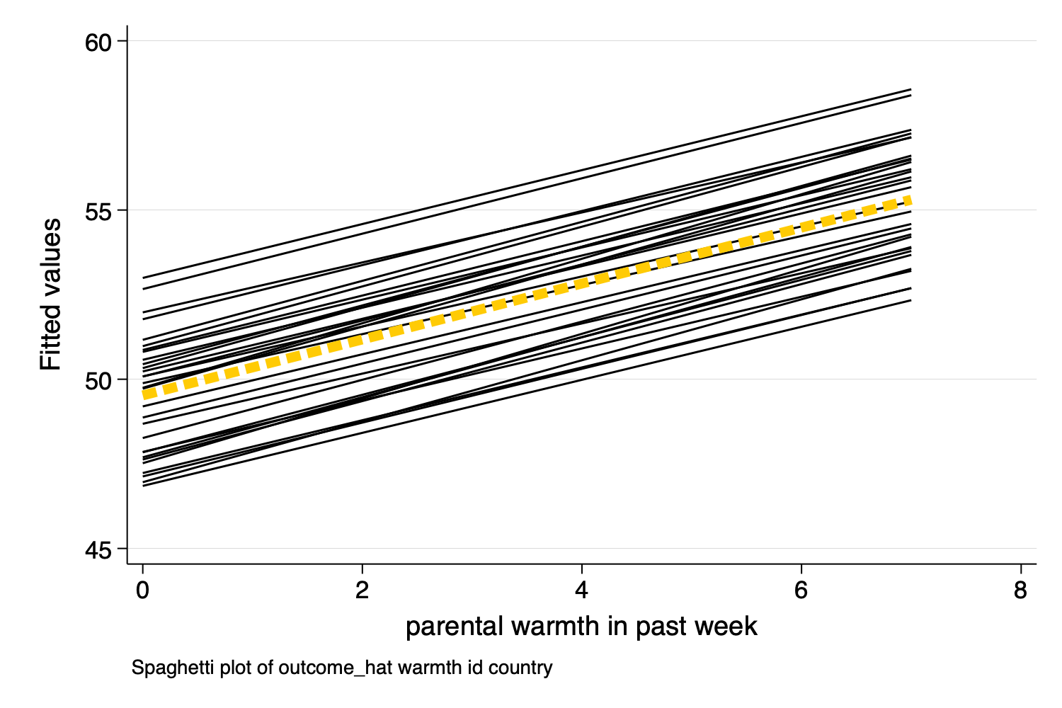
Figure 10: Spaghetti Plot With Predicted Values
margins and marginsplotIn contrast to predict, which generates a predicted
value for every observation in the data, margins
generates predicted values at specific values of certain
variables.
Performing EM optimization ...

Performing gradient-based optimization:
Iteration 0:  Log likelihood = -9628.1621
Iteration 1:  Log likelihood = -9628.1621

Computing standard errors ...

Mixed-effects ML regression                          Number of obs    =  3,000
Group variable: country                              Number of groups =     30
                                                     Obs per group:
                                                                  min =    100
                                                                  avg =  100.0
                                                                  max =    100
                                                     Wald chi2(3)     = 370.90
Log likelihood = -9628.1621                          Prob > chi2      = 0.0000

------------------------------------------------------------------------------------
           outcome | Coefficient  Std. err.      z    P>|z|     [95% conf. interval]
-------------------+----------------------------------------------------------------
            warmth |   .8330937   .0574809    14.49   0.000     .7204332    .9457543
physical_punishm~t |  -.9937819   .0798493   -12.45   0.000    -1.150284   -.8372801
    1.intervention |   .6406043   .2175496     2.94   0.003      .214215    1.066994
             _cons |   51.65238   .4664841   110.73   0.000     50.73809    52.56668
------------------------------------------------------------------------------------

------------------------------------------------------------------------------
  Random-effects parameters  |   Estimate   Std. err.     [95% conf. interval]
-----------------------------+------------------------------------------------
country: Identity            |
                  var(_cons) |   3.371762   .9613269      1.928279    5.895816
-----------------------------+------------------------------------------------
               var(Residual) |    35.0675    .910002      33.32853    36.89721
------------------------------------------------------------------------------
LR test vs. linear model: chibar2(01) = 204.14 Prob >= chibar2 = 0.0000marginsPredictive margins Number of obs = 3,000
Expression: Linear prediction, fixed portion, predict()
1._at: warmth = 1
2._at: warmth = 2
3._at: warmth = 3
4._at: warmth = 4
5._at: warmth = 5
6._at: warmth = 6
7._at: warmth = 7
----------------------------------------------------------------------------------
| Delta-method
| Margin std. err. z P>|z| [95% conf. interval]
-----------------+----------------------------------------------------------------
_at#intervention |
1 0 | 50.02222 .3966755 126.10 0.000 49.24475 50.79969
1 1 | 50.66283 .3955286 128.09 0.000 49.88761 51.43805
2 0 | 50.85532 .3788571 134.23 0.000 50.11277 51.59786
2 1 | 51.49592 .3789096 135.91 0.000 50.75327 52.23857
3 0 | 51.68841 .3692182 139.99 0.000 50.96476 52.41207
3 1 | 52.32902 .370554 141.22 0.000 51.60274 53.05529
4 0 | 52.52151 .3684014 142.57 0.000 51.79945 53.24356
4 1 | 53.16211 .3710204 143.29 0.000 52.43492 53.8893
5 0 | 53.3546 .376464 141.73 0.000 52.61674 54.09246
5 1 | 53.9952 .3802764 141.99 0.000 53.24988 54.74053
6 0 | 54.18769 .3928599 137.93 0.000 53.4177 54.95768
6 1 | 54.8283 .3977088 137.86 0.000 54.0488 55.60779
7 0 | 55.02079 .4166062 132.07 0.000 54.20425 55.83732
7 1 | 55.66139 .4223062 131.80 0.000 54.83369 56.4891
----------------------------------------------------------------------------------marginsplot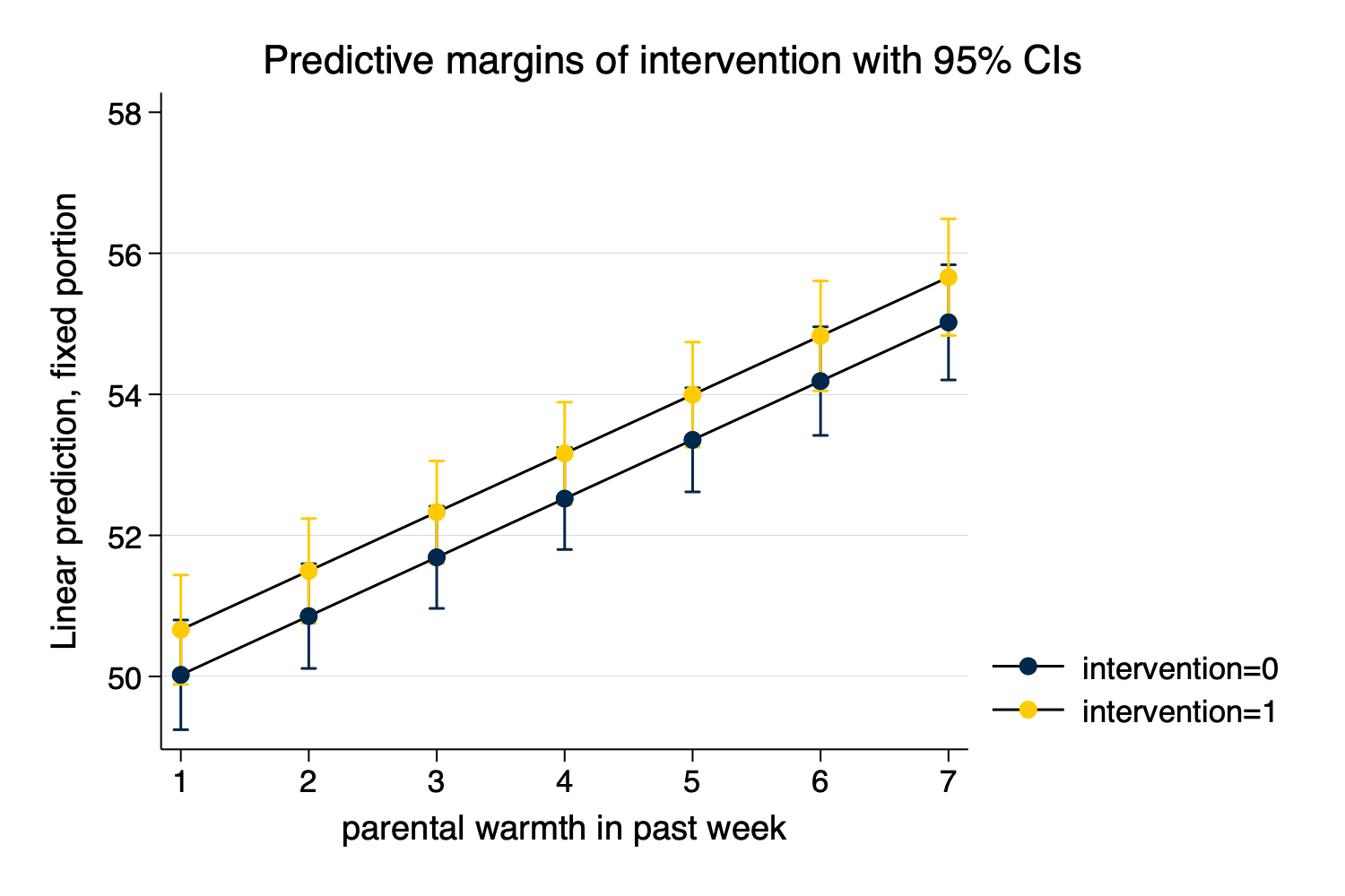
Figure 11: Predicted Values From margins and
marginsplot
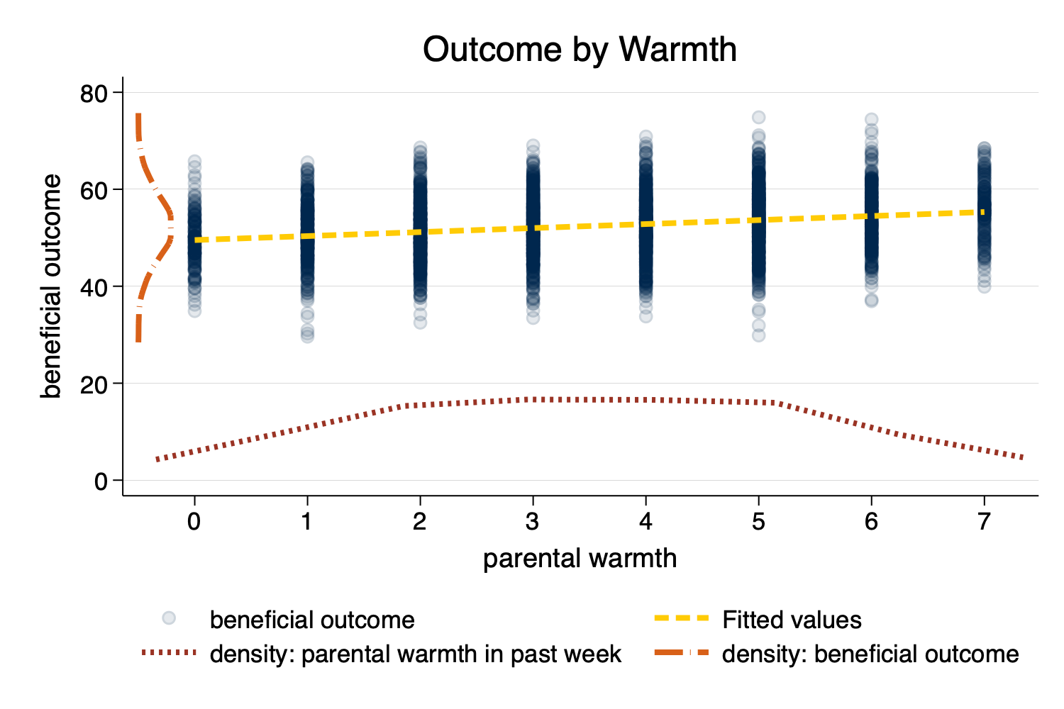
twoway ...)[!NOTE]
You may have to experiment with whether scatterplots or line plots work best for displaying the x and y densities.
twoway (scatter outcome warmth, mcolor(%10)) /// scatterplot w some transparency
(lfit outcome warmth) /// linear fit
(line warmth_d warmth_x) /// line plot of x density
(line outcome_y outcome_d), /// line plot of y density (note flipped order)
title("Outcome by Warmth") /// title
ytitle("beneficial outcome") /// manual ytitle
xtitle("parental warmth") /// manual xtitle
legend(position(6) rows(2) ) /// legend at bottom; 2 rows
xlabel(0 1 2 3 4 5 6 7) /// manual x labels
name(mynewscatter, replace)

graph export mynewscatter.png, width(1500) replace