use "FrenchSkiiers.dta"From Contingency Table To Logistic Regression
With the French Skiiers Data
1 The Data
We use the French Skiiers data that we have used in other examples.
2 Contingency Table
tabulate Tx Outcome [fweight = Count] | Outcome
Tx | No Cold Cold | Total
--------------+----------------------+----------
Placebo | 109 31 | 140
Ascorbic Acid | 122 17 | 139
--------------+----------------------+----------
Total | 231 48 | 279 For the sake of teaching and exposition, I re-arrange the numbers slightly.
| Develop Outcome | Do Not Develop Outcome | |
|---|---|---|
| Exposed | a | b |
| Not Exposed | c | d |
| Cold | No Cold | |
|---|---|---|
| Ascorbic Acid | 17 (a) | 122 (b) |
| Placebo | 31 (c) | 109 (d) |
2.1 Risk (\(R\)) and Risk Differences (\(RD\))
\(R = \frac{a}{a+b}\) (in Exposed)
\(RD =\)
\(\text{risk in exposed} - \text{risk in not exposed} =\)
\(a/(a+b) - c/(c+d) =\)
\((17/139) - (31/140) =\)
\(-.09912641\)
How do we talk about this risk difference?
2.2 Odds Ratios (\(OR\))
| Develop Outcome | Do Not Develop Outcome | |
|---|---|---|
| Exposed | a | b |
| Not Exposed | c | d |
\(OR =\)
\(\frac{\text{odds that exposed person develops outcome}}{\text{odds that unexposed person develops outcome}} =\)
\(\frac{\frac{a}{a+b} / \frac{b}{a+b}}{\frac{c}{c+d} / \frac{d}{c+d}} =\)
\(\frac{a/b}{c/d} =\)
\(\frac{ad}{bc} =\)
\((17 * 109)/(122 * 31) =\)
\(.4899526\)
How do we talk about this odds ratio?
3 Logistic Regression
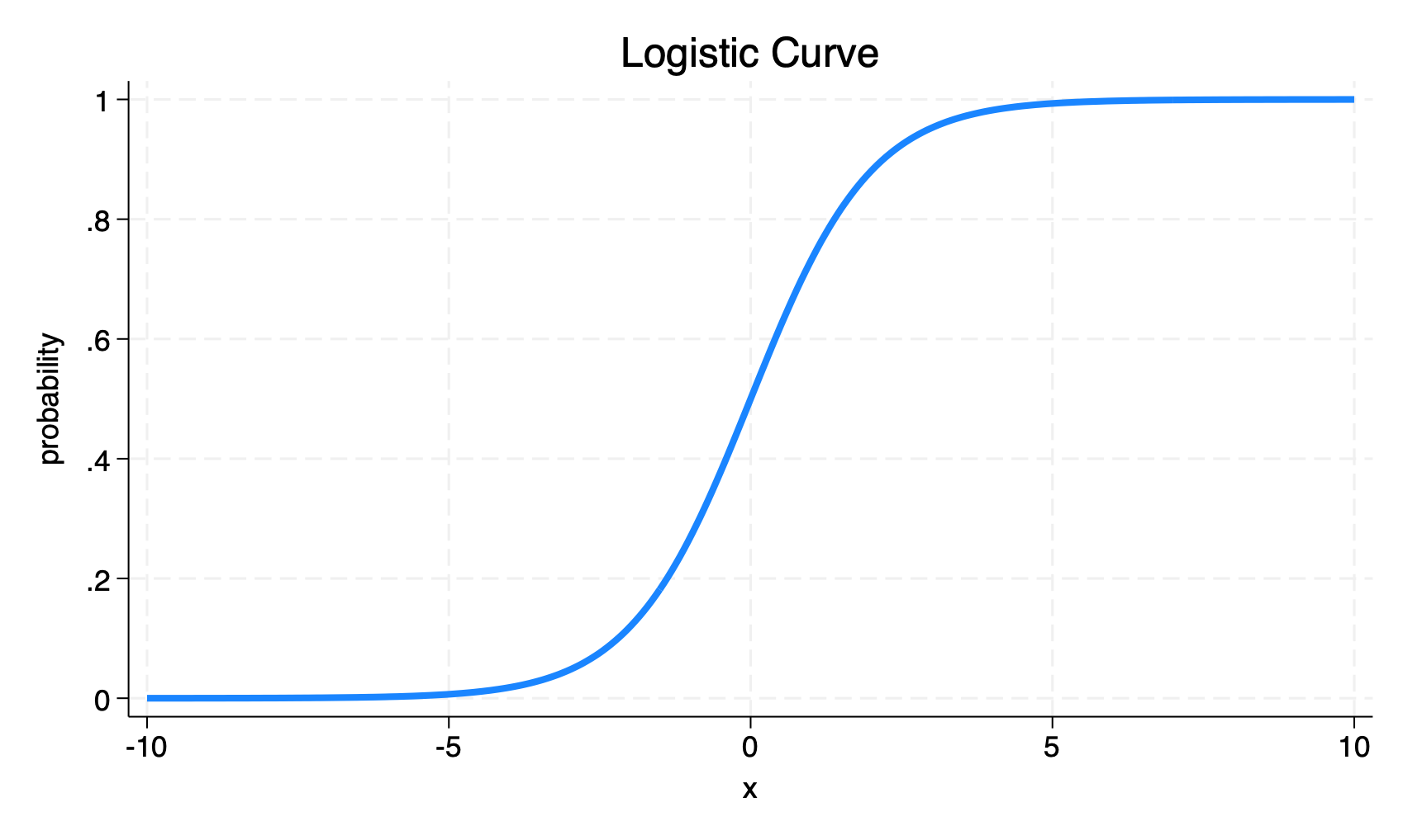
As discussed, the formula for logistic regression is:
\[\ln \Big(\frac{p(\text{outcome})}{1-p(\text{outcome})} \Big) = \beta_0 + \beta_1 x\]
Here \(p(\text{outcome})\) is the probability of the outcome.
\(\frac{p(\text{outcome})}{1-p(\text{outcome})}\) is the odds of the outcome.
Hence, \(\ln \Big(\frac{p(\text{outcome})}{1-p(\text{outcome})} \Big)\)1 is the log odds of the outcome.
The logistic regression equation has the desired functional form.
The logistic regression equation is appropriate to reflect changes in the probability of an outcome that can be either 1 or 0.
Logistic regression returns a \(\beta\) coefficient for each independent variable \(x\).
These \(\beta\) coefficients can then be exponentiated to obtain odds ratios: \(OR = e^{\beta}\)
Exponentiation “undoes” the logarithmic transformation.
If \(\ln(y) = x\), then \(y = e^x\)
So, if … \(\ln \Big(\frac{p(\text{outcome})}{1-p(\text{outcome})}\Big) = \beta_0 + \beta_1 x\) then \(\frac{p(\text{outcome})}{1-p(\text{outcome})} = e^{\beta_0 + \beta_1 x} = e^{\beta_0} \times e^{\beta_1 x}\)
We see that the odds ratio given by logistic regression,
.4899526, is the exact same as that given by manually calculating the odds ratio from a contingency table.
An advantage of logistic regression is that it can be extended to multiple independent variables.
logit Outcome Tx [fweight = Count], orIteration 0: Log likelihood = -128.09195
Iteration 1: Log likelihood = -125.68839
Iteration 2: Log likelihood = -125.65611
Iteration 3: Log likelihood = -125.6561
Logistic regression Number of obs = 279
LR chi2(1) = 4.87
Prob > chi2 = 0.0273
Log likelihood = -125.6561 Pseudo R2 = 0.0190
------------------------------------------------------------------------------
Outcome | Odds ratio Std. err. z P>|z| [95% conf. interval]
-------------+----------------------------------------------------------------
Tx | .4899526 .1613519 -2.17 0.030 .256942 .9342712
_cons | .2844037 .0578902 -6.18 0.000 .1908418 .423835
------------------------------------------------------------------------------
Note: _cons estimates baseline odds.How do we talk about this odds ratio? How would we talk about it if it was \(> 1.0\)? \(> 2.0\)
4 Measures of Effect Size
Effect Sizes
Think about the risk difference, the risk ratio, and the odds ratio. What measure gives the most substantively accurate sense of the size of the effect? What measures may possibly overstate the effect.
Footnotes
It is sometimes useful to think of the log odds as a transformed dependent variable. We have transformed the dependent variable so that it can be expressed as a linear function of the independent variables, e.g.: \(\beta_0 + \beta_1 x\)↩︎