Show the code
twoway function y = 2 * x, lwidth(thick) ///
title("Linear Function") subtitle("With Coefficient 2") ///
range(-10 10)

graph export linear0.png, replaceWe begin with the linear function:
\[y = ax\]
The coefficient a tells us how much y increases for a 1 unit increase in x.
twoway function y = 2 * x, lwidth(thick) ///
title("Linear Function") subtitle("With Coefficient 2") ///
range(-10 10)
graph export linear0.png, replace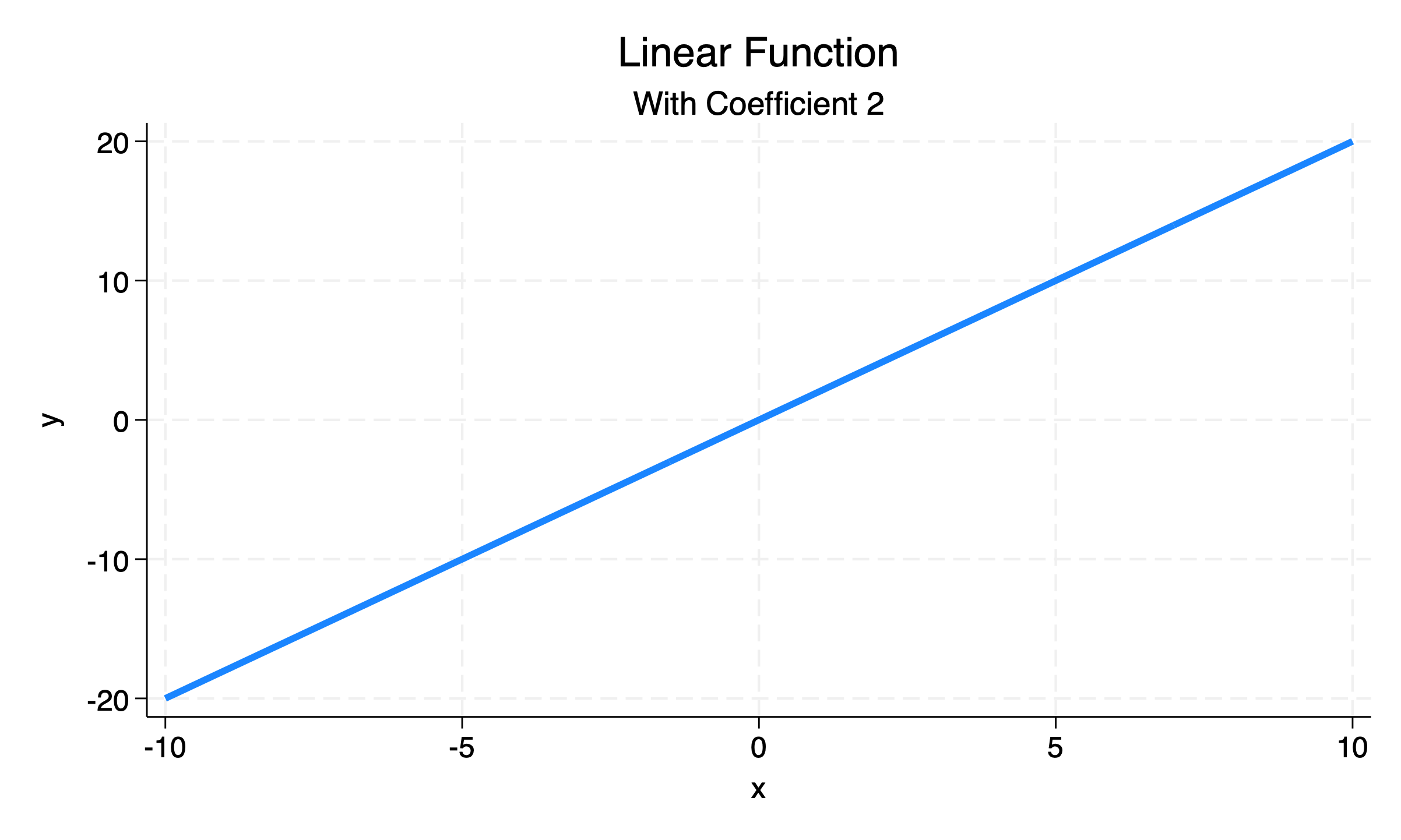
We then introduce the exponential function:
\[y = \text{base}^{\text{exponent}}\]
The exponent tells us how many times to multiply the base by itself to get the result.
For example: \(2^3 = 8\) because \(2 \times 2 \times 2 = 8\)
twoway function y = 2^x, lwidth(thick) ///
title("Exponential Function") subtitle("With Base 2") ///
range(-10 10)

graph export exponential0.png, replace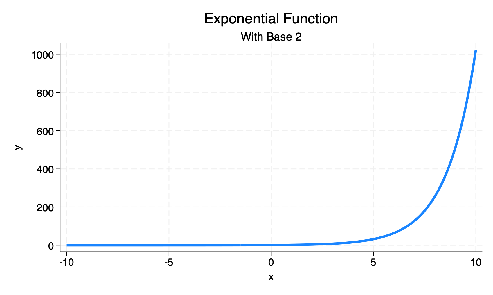
Exponential functions–and hence their inverses, logarithmic functions described below–have applications in the study of categorical data analysis, radioactive decay, disease spread, and population growth.
We then consider the logarithm.
If \[y = b^x\] then \[\log_b(y) = x\]
In words: If \(\text{number} = \text{base}^{\text{exponent}}\) then \(\log_{\text{base}}(\text{number}) = \text{exponent}\).
For example, \(2^3 = 8\), therefore \(log_2 8 = 3\).
The logarithm answers the question: What is the power to which we have to raise the number to get the result?
The logarithm may thus be thought of as the inverse of the exponential function.
twoway function y = ln(x)/ln(2), lwidth(thick) ///
title("Logarithmic Function") subtitle("Base 2") ///
range(-10 10)

graph export logarithmic0.png, replace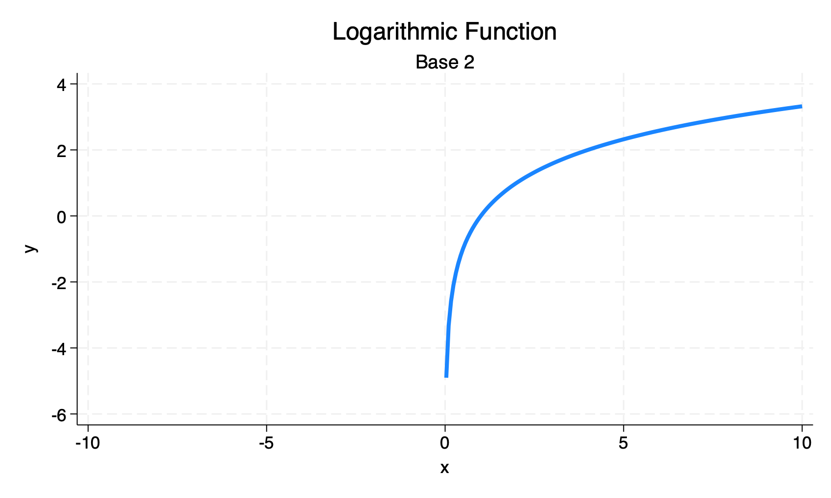
For deep mathematical reasons, it is often useful to use logarithms with base \(e\) which is often termed the natural logarithm, written \(\ln\)
\(e\) is a kind of fundamental mathematical constant, like \(\pi\), but without the easy geometric definition that \(\pi\) has. (For any \(\bigcirc\), \(\pi = \frac{\text{circumference}}{\text{diameter}}\).)
\(e\) emerges in many contexts, including some aspects of compound growth processes 1. \(e\) is approximately equal to 2.71828….
If \[y = e^x\] then \[\ln(y) = x\]
twoway function y = exp(x), lwidth(thick) ///
title("Exponential Function") subtitle("Base e") ///
range(-10 10)

graph export exponential.png, replace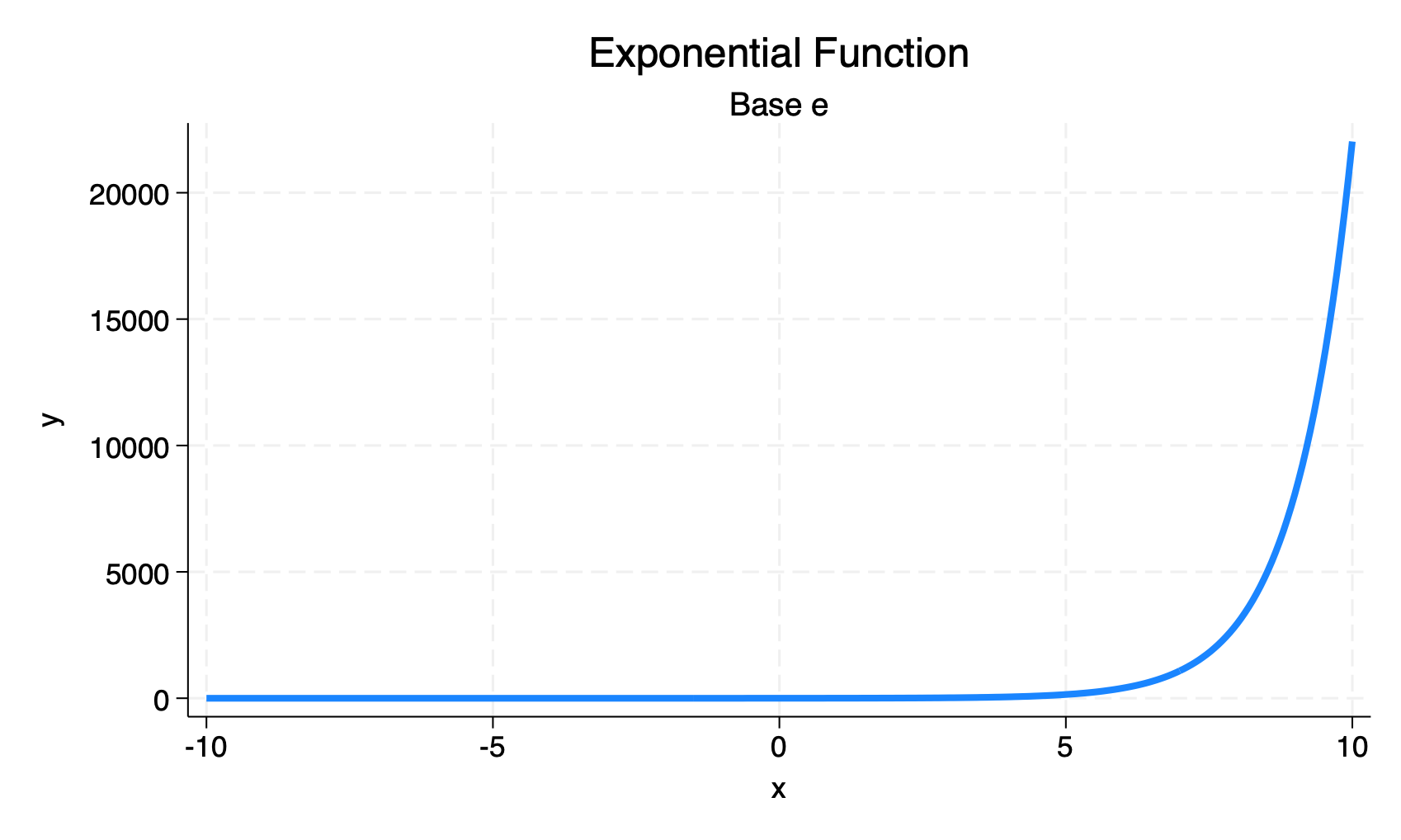
twoway function y = ln(x), lwidth(thick) ///
title("Logarithmic Function") subtitle("Base e") ///
range(-10 10)

graph export logarithmic.png, replace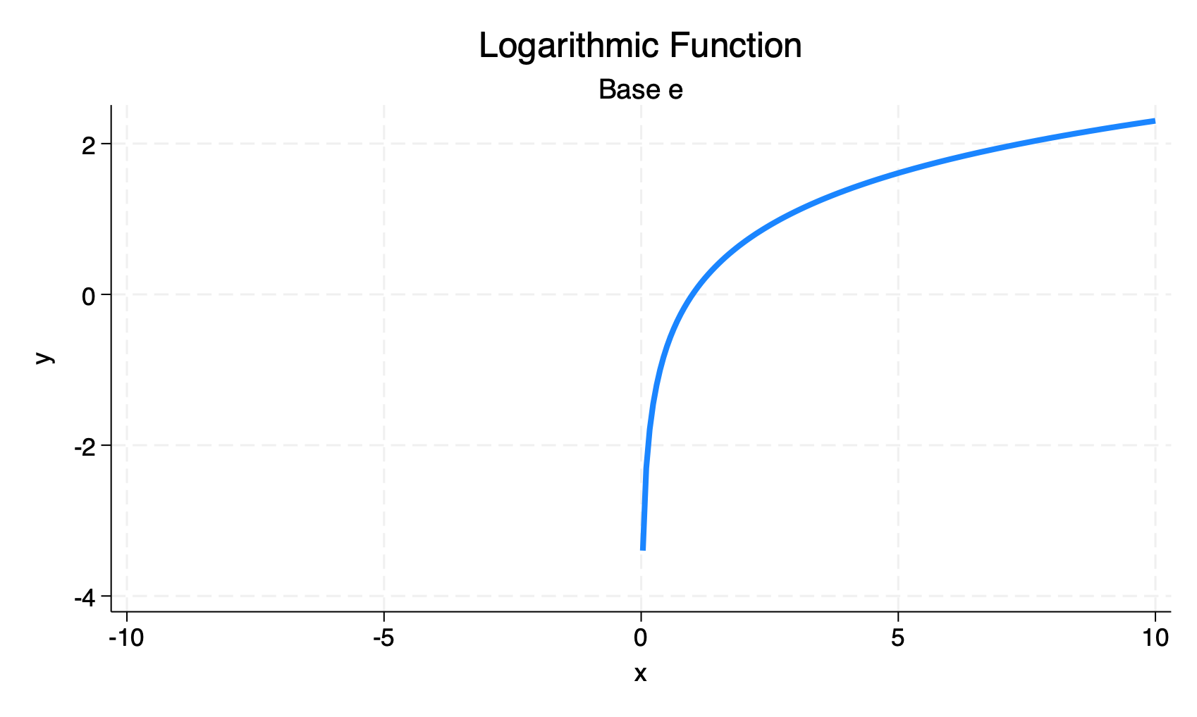
In categorical data analysis–especially later in the course–we are often thinking about some equation like \(\ln(y) = \beta x\). This is equivalent to \(y = e^{\beta x}\) so many models–particularly later in the course–will have us thinking about exponential relationships.
Early on in this course, we will think about logistic regression. In logistic regression, we start by thinking about the odds of our outcome:
\[\frac{p(y)}{1-p(y)}\]
We will ultimately be working with the logarithm of the odds, or the log odds:
\[\ln(\frac{p(y)}{1-p(y)}) = x\]
To graph these log odds, we need to solve for \(p(y)\):
\[p(y) = \frac{e^x}{1 + e^x}\]
twoway function y = exp(x)/(1 + exp(x)), lwidth(thick) ///
title("Logistic Function") ///
range(-10 10)

graph export logistic.png, replace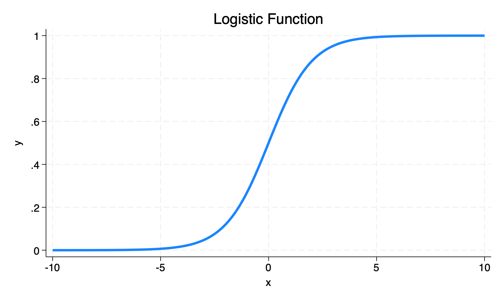
This function is sometimes called a sigmoid, and has the interesting property of mapping the interval \(- \infty < x < \infty\) to \(0 < y < 1\). (This is the first step in mapping a continuous predictor to a categorical outcome.)
An interesting sidenote is that the logarithm forms the basis of the logarithmic spiral. The equation for a logarithmic spiral in polar coordinates is: \(r = ae^{b \theta}\), where \(\theta\) is the angle, \(r\) is the radius, and \(a\) and \(b\) are constants.
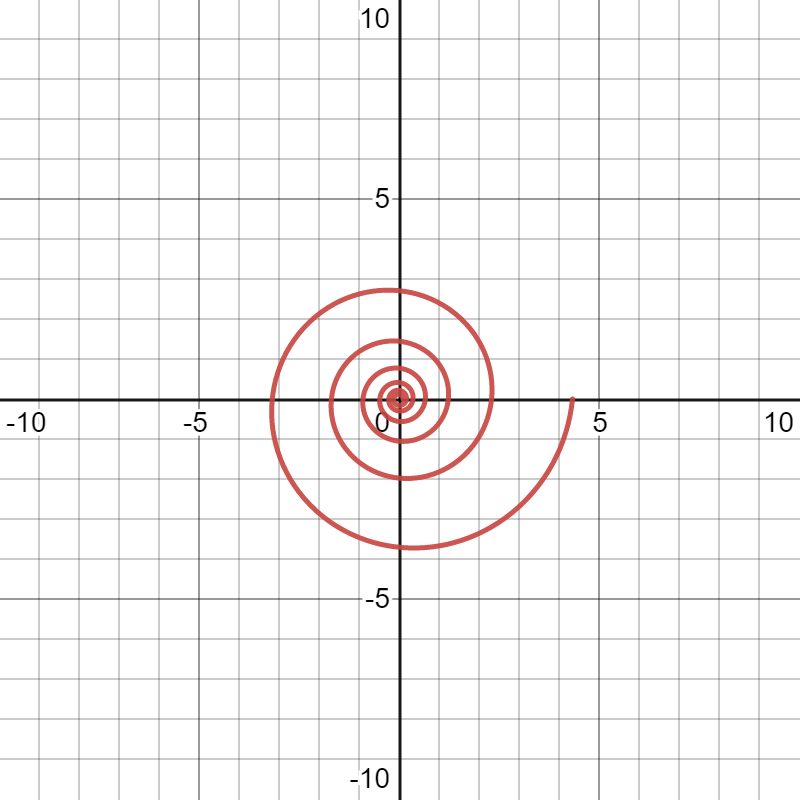
Logarithmic spirals can be found in nature in the nautilus shell, and in sunflowers and in the flight of hawks.
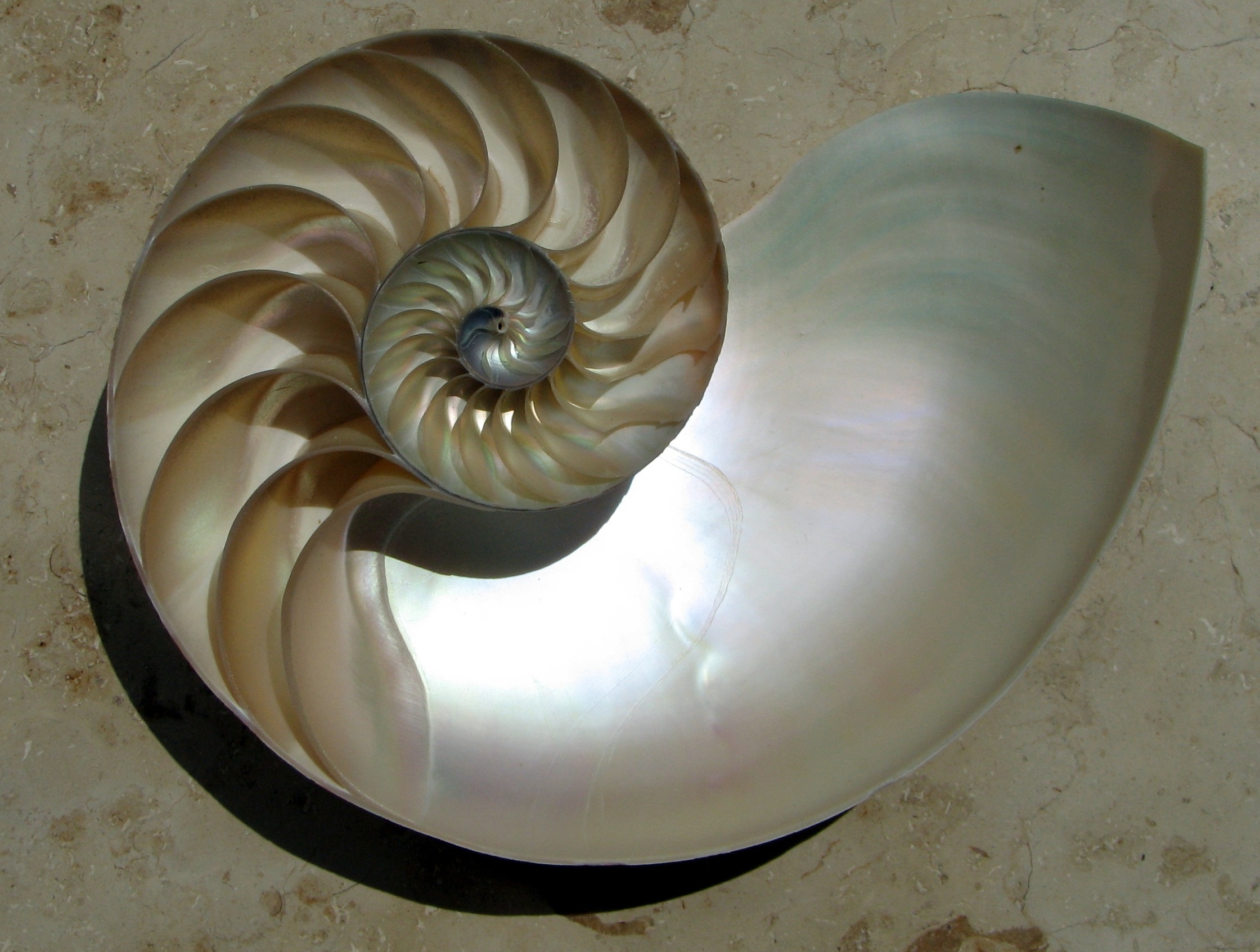

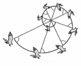
Logarithmic Spirals
A common definition of \(e\) is \[e = \lim_{n \to \infty} \left(1 + \frac{1}{n} \right)^n\]↩︎