Introduction

“Survival analysis is a key technique in data-driven decision-making, which is now central to public interest because of COVID-19. Applying the correct technique for the specific question at hand is crucial for credible public health inferences. If you are interested in assessing how a risk factor or a potential treatment affects the progression of a disease—such as how long a patient takes to recover—then survival analysis techniques come into play. Survival analysis deeply respects the ultimate source of its data, often the disease experience or even the life and death of human patients. It seeks to exploit every last drop of information that this experience can render for saving lives—in particular, not only whether patients survived, but how long, and why. And it strives to do so with minimal assumptions, so that the data are truly driving the decision.”

—SAS Corporation

Key Concepts

WHO CARES how we measure time? Isn’t it self-evident?

Implementations differ; formulas are our friends
\(h(t) = x1 + x2 + \text{etc.} ...\): formula (effect on hazard (instantaneous rate of occurrence))

The “Hospital Bed Problem”

Imagine a Hypothetical Hospital
Imagine that there are 52 patients total.
51 of the patients are long term patients, who each stay for 1 year.
1 of the patients is a short term patient, who stays for 1 week.

Is this a hospital that serves mostly long-term, or short term patients?

. clear all

. set obs 52 // 52 hypothetical obervations
Number of observations (_N) was 0, now 52.

. generate id = _n // set id = to observation #

. generate weeks = 52

. replace weeks = 1 if id == 52
(1 real change made)

. twoway (scatter id weeks if weeks == 52, msize(small)) /// staying 52 weeks
> (scatter id weeks if weeks == 1, msize(small)), /// staying 1 week
> title("Hypothetical Hospital") ///
> legend(on order(1 "long term" 2 "short term")) ///
> xtitle("week of discharge") ///
> ylabel(1(1)52, labels labsize(tiny) angle(horizontal) noticks nogrid) /// 
> scheme(michigan)

. graph export hospital_bed_problem.png, width(1000) replace
file
    /Users/agrogan/Desktop/newstuff/categorical/survival-analysis-and-event-history/hospital_bed_p
    > roblem.png saved as PNG format

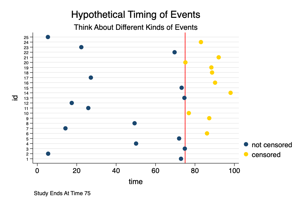
Illustration of Hospital Bed Problem

How To Measure Length of Stay (1)

. clear all

. set obs 25 // 25 hypothetical obervations
Number of observations (_N) was 0, now 25.

. generate id = _n // set id = to observation #

. generate time = runiform(1, 100) // random times

. generate censored = time > 75 // censored if time > 75

. twoway (scatter id time if censored == 0) ///
> (scatter id time if censored == 1), ///
> title("Hypothetical Timing of Events") ///
> subtitle("Think About Different Kinds of Events") ///
> note("Study Ends At Time 75") ///
> legend(on order(1 "not censored" 2 "censored")) ///
> xline(75, lcolor("red")) /// censoring line at 75
> ylabel(1(1)25, labsize(vsmall) angle(horizontal)) /// lines from 1 to 25
> scheme(michigan)

. graph export timing_of_events.png, width(1000) replace
file
    /Users/agrogan/Desktop/newstuff/categorical/survival-analysis-and-event-history/timing_of_even
    > ts.png saved as PNG format

Timing Of Events

Animated

See times-events-and-censoring.html

How To Measure Length of Stay (2)

Event happened within a specified time (yes/no)

\[ \ln(\frac{P(\text{event})}{1-P(\text{event})}) = \beta_0 + \beta_1 x_1 + \beta_2 x_2 + e_i \]

Statistically accurate, but we lose information on when the event happened.
Statistically less efficient.

Time until Event

\[ \text{time until event} = \beta_0 + \beta_1 x_1 + \beta_2 x_2 + e_i \]

What to do with events that haven’t happened yet? (Censoring)
Code as missing. Loss of information if using complete cases. Possible bias.
Code as 0. Possible bias. They might happen at some point.
Code as time of censoring. Possible bias. They might never happen. They might happen much later.

Hazard (Risk) of Event Occurence

A more heuristic definition:

\[ h(t) = \lim_{\delta\to 0} \frac{\text{probability of having an event before time } t + \delta}{\delta} \]

This definition per Johnson & Shih (2007)

A more formal definition:

\[ h(t) = \lim_{\Delta t \to 0} \frac{P(t \le T < t + \Delta t | T > t)}{\Delta t} \]

This definition per Ragnar Frisch Centre for Economic Research (2020)

A Policy Example (Welfare Reform, 1996)

From LaDonna Pavetti (1995)

time in months
new entrants (percent)
all current recipients at a point in time (percent)

. clear all

. use Pavetti.dta
(Written by R.              )

. list, abbreviate(25) // list out the data

     ┌─────────────────────────────────────────────────┐
     │    time   new_entrants   all_current_recipients │
     ├─────────────────────────────────────────────────┤
  1. │    1-12           27.4                      4.5 │
  2. │   13-24           14.8                      4.8 │
  3. │   25-36             10                      4.9 │
  4. │   37-48            7.7                        5 │
  5. │   49-60            5.5                      4.5 │
     ├─────────────────────────────────────────────────┤
  6. │ Over 60           34.6                     76.3 │
     └─────────────────────────────────────────────────┘

. graph bar (asis) all_current_recipients, /// this particular set of options was difficult to figur
> e out!
> asyvars ///
> over(time) ///
> title("All Current Recipients") ///
> sub("By Months On Caseload") ///
> ytitle("percent") ///
> scheme(michigan)

. graph export all_current_recipients.png, width(1000) replace
file
    /Users/agrogan/Desktop/newstuff/categorical/survival-analysis-and-event-history/all_current_re
    > cipients.png saved as PNG format

All Current Recipients by Months on Caseload

Welfare Reform (2)

. graph bar (asis) new_entrants, ///
> asyvars ///
> over(time) ///
> title("New Recipients") ///
> sub("By Months On Caseload") ///
> ytitle("percent") ///
> scheme(michigan)

. graph export new_recipients.png, width(1000) replace
file
    /Users/agrogan/Desktop/newstuff/categorical/survival-analysis-and-event-history/new_recipients
    > .png saved as PNG format

New Recipients by Months on Caseload

Survival Analysis and Event History

References

Johnson, L. L., & Shih, J. H. (2007). CHAPTER 20 - An Introduction to Survival Analysis (J. I. Gallin & F. P. Ognibene, eds.). https://doi.org/https://doi.org/10.1016/B978-012369440-9/50024-4
Ragnar Frisch Centre for Economic Research (2020). Event History Analysis, Survival Analysis, Duration Analysis ,Transition Data Analysis, Hazard Rate Analysis. Oslo, Norway.