use simulated_multilevel_data.dta, clearIn another post, I mentioned that for a few recent projects, I have had to quickly get up to speed on new data. In that other post, I focused on the idea of using a pairs plot in R.
In this post, I want to focus on a similar idea. But instead of a pairs plot, I focus on using a regression model with a number of risk and protective factors predicting an outcome. Here I use Stata instead of R, and use Stata’s powerful margins and marginsplot commands to get a visual idea of the way that these different risk and protective factors are associated with the outcome.
Using margins means that I’m going to use some complicated looking syntax to get some results that are actually pretty straightforward.
For this example, I use the data from my Multilevel Workshop site.
Get The Data
describe The Data
describeRunning /Users/agrogan/Desktop/GitHub/agrogan1.github.io/posts/exploring-data/profile.do ..
> .
Contains data from simulated_multilevel_data.dta
Observations: 3,000
Variables: 9 15 May 2024 14:54
-------------------------------------------------------------------------------------------
Variable Storage Display Value
name type format label Variable label
-------------------------------------------------------------------------------------------
country float %9.0g country id
HDI float %9.0g Human Development Index
family float %9.0g family id
id str7 %9s unique country family id
identity float %9.0g hypothetical identity group variable
intervention float %9.0g recieved intervention
physical_puni~t float %9.0g physical punishment in past week
warmth float %9.0g parental warmth in past week
outcome float %9.0g beneficial outcome
-------------------------------------------------------------------------------------------
Sorted by: country familyRegression Model (mixed or regress)
Because these data are clustered by country, I use the mixed command to get accurate standard errors and p values.
mixed outcome warmth physical_punishment i.intervention i.identity || country:
NoteShow The Results
Running /Users/agrogan/Desktop/GitHub/agrogan1.github.io/posts/exploring-data/profile.do ..

> .


Performing EM optimization ...

Performing gradient-based optimization:
Iteration 0:  Log likelihood = -9627.1393
Iteration 1:  Log likelihood = -9627.1393

Computing standard errors ...

Mixed-effects ML regression                          Number of obs    =  3,000
Group variable: country                              Number of groups =     30
                                                     Obs per group:
                                                                  min =    100
                                                                  avg =  100.0
                                                                  max =    100
                                                     Wald chi2(4)     = 373.21
Log likelihood = -9627.1393                          Prob > chi2      = 0.0000

-------------------------------------------------------------------------------------
            outcome | Coefficient  Std. err.      z    P>|z|     [95% conf. interval]
--------------------+----------------------------------------------------------------
             warmth |   .8342119   .0574661    14.52   0.000     .7215805    .9468434
physical_punishment |  -.9934352   .0798217   -12.45   0.000    -1.149883   -.8369874
     1.intervention |   .6462874   .2175097     2.97   0.003     .2199762    1.072598
         1.identity |  -.3104984   .2170594    -1.43   0.153    -.7359271    .1149302
              _cons |   51.79936   .4777788   108.42   0.000     50.86293    52.73579
-------------------------------------------------------------------------------------

------------------------------------------------------------------------------
  Random-effects parameters  |   Estimate   Std. err.     [95% conf. interval]
-----------------------------+------------------------------------------------
country: Identity            |
                  var(_cons) |   3.377381   .9627211      1.931725    5.904929
-----------------------------+------------------------------------------------
               var(Residual) |   35.04285   .9093623       33.3051    36.87127
------------------------------------------------------------------------------
LR test vs. linear model: chibar2(01) = 204.68        Prob >= chibar2 = 0.0000
Were the data not clustered, I could have just as easily used regress.
regress outcome warmth physical_punishment i.intervention i.identity
Use margins to Get Marginal Effects
margins in Stata is a very versatile (and sometimes confusing) command. Here I use slightly complicated syntax, to get a very simple set of results. I use margins, and the dydx(*) option to get marginal effects, which here are simply the \(\beta\) coefficients reported above.
TipWhy Go Through This Step?
We want to “let margins”know” about the regression coefficients”.
As we will see below, letting margins calculate the regression coefficients lets us graph the results using marginsplot.
TipTechnically Speaking…
Technically speaking, dydx(*) is asking Stata to calculate the marginal effects, \(\frac{\partial y}{\partial x}\) for all (*) independent variables in the model. In a linear model, with no interaction terms, \(\frac{\partial y}{\partial x} = \beta\).
Again, we are essentially using slightly complicated syntax to get simple results.
margins, dydx(*)Running /Users/agrogan/Desktop/GitHub/agrogan1.github.io/posts/exploring-data/profile.do ..
> .
Average marginal effects Number of obs = 3,000
Expression: Linear prediction, fixed portion, predict()
dy/dx wrt: warmth physical_punishment 1.intervention 1.identity
-------------------------------------------------------------------------------------
| Delta-method
| dy/dx std. err. z P>|z| [95% conf. interval]
--------------------+----------------------------------------------------------------
warmth | .8342119 .0574661 14.52 0.000 .7215805 .9468434
physical_punishment | -.9934352 .0798217 -12.45 0.000 -1.149883 -.8369874
1.intervention | .6462874 .2175097 2.97 0.003 .2199762 1.072598
1.identity | -.3104984 .2170594 -1.43 0.153 -.7359271 .1149302
-------------------------------------------------------------------------------------
Note: dy/dx for factor levels is the discrete change from the base level.Use marginsplot To Visualize the Marginal Effects
First I use marginsplot with no options to visualize the marginal effects. This produces a pretty non-intuitive graph.
marginsplot

graph export "marginsplot1.png", replace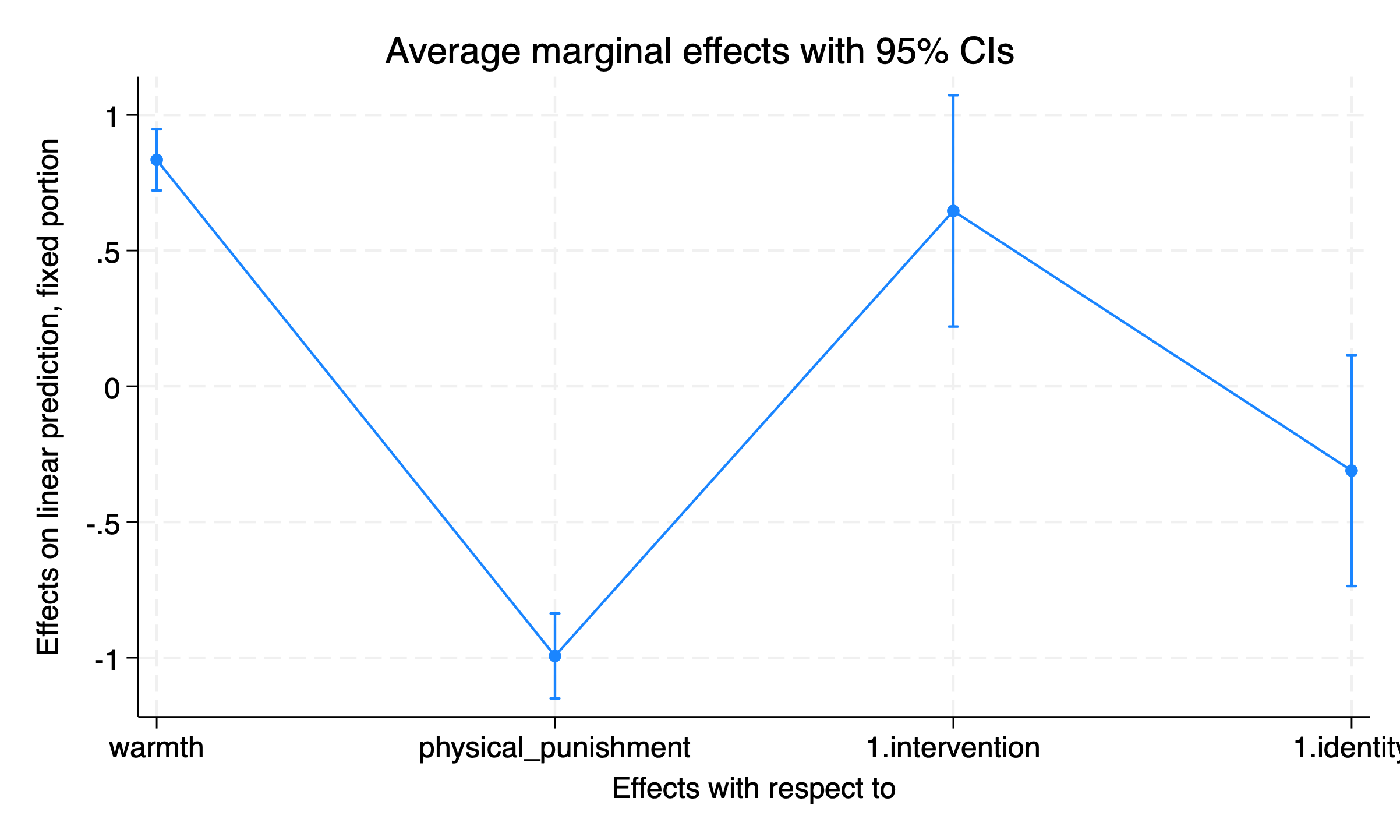
marginsplot with default optionsUse marginsplot With Better Options
I add some options to clarify the graph. I recast the graph as a scatterplot. I flip the graph to be horizontal. I also add a reference line at \(x = 0\) to make more clear which coefficients are significant, and which coefficients are not significant.
marginsplot, ///
recast(scatter) /// recast as scatterplot
horizontal /// flip to horizontal
xline(0, lcolor(red)) // line at x = 0 in red

graph export "marginsplot2.png", replace
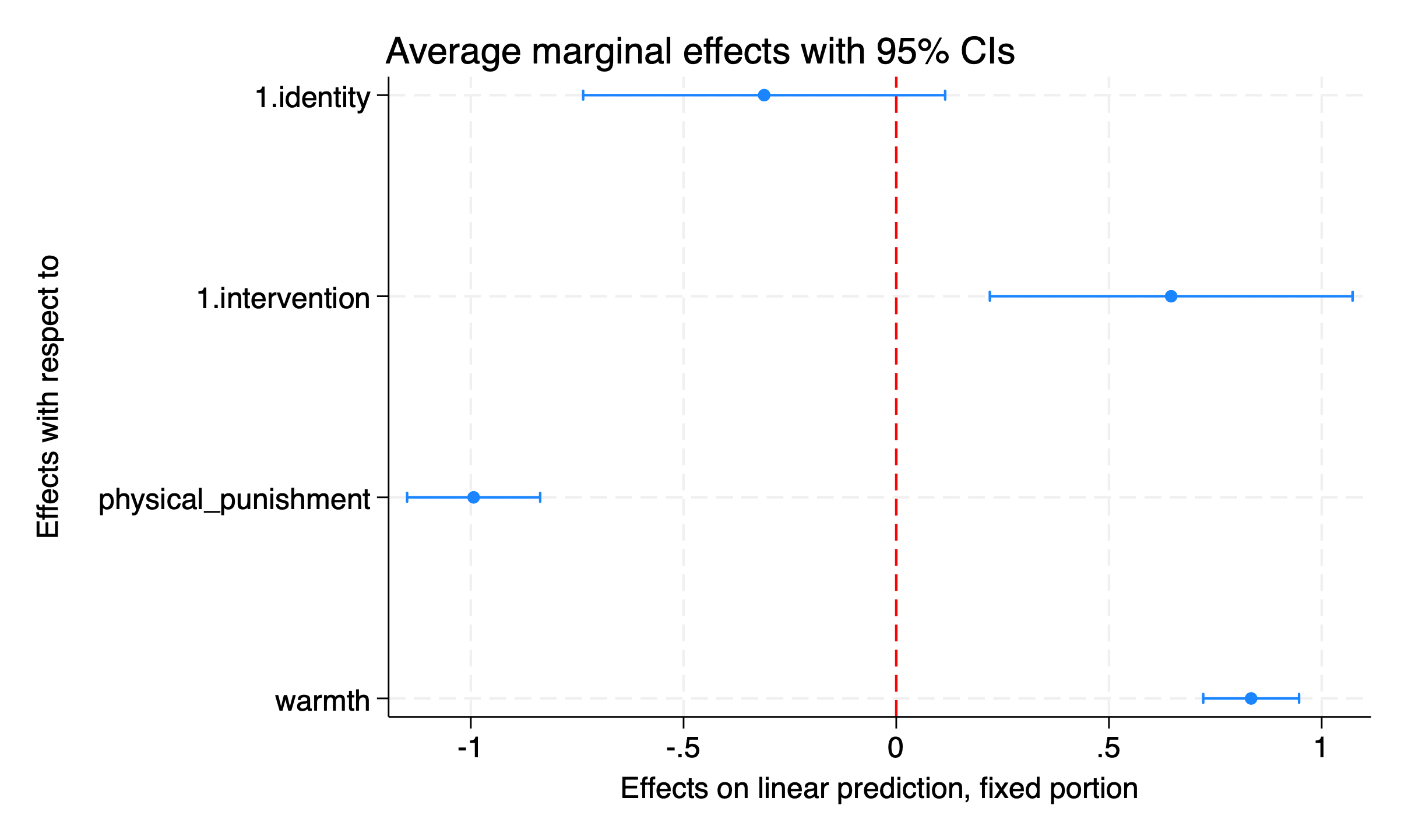
marginsplot with better optionsConclusion
In conclusion:
- I ran a regression model using
mixed(I could have usedregress). - I transferred the values of the \(\beta\) regression coefficients to
margins. - I used
marginsplotwith a few options to see the results.
These steps: mixed or regress; margins; marginsplot, could be repeated for almost any analysis.
Results suggest that identity is not associated with the outcome. The intervention is associated with improvements in the outcome. physical_punishment is associated with a worsened outcome. Parental warmth is associated with an improved outcome.