set linesize 80 // set linesize for nice formatting

use "simulated_multilevel_data.dta", clear4 Two Level Cross Sectional; And Three Level Longitudinal Models
4.1 Cross Sectional Model
4.1.1 Get Data
library(haven)

simulated_multilevel_data <- read_dta("simulated_multilevel_data.dta")
4.1.2 The Equation
\[\begin{aligned} \text{outcome}_{ij} = \beta_0 + \beta_1 \text{parental warmth} + \beta_2 \text{physical punishment} + \\ \beta_3 \text{identity} + \beta_4 \text{intervention} + \beta_5 HDI + \\ u_{0j} + u_{1j} \times \text{parental warmth} + e_{ij} \end{aligned} \tag{4.1}\]
4.1.3 Descriptive Statistics
summarize // descriptive statistics Variable | Obs Mean Std. dev. Min Max
-------------+---------------------------------------------------------
country | 3,000 15.5 8.656884 1 30
HDI | 3,000 64.76667 17.24562 33 87
family | 3,000 50.5 28.87088 1 100
id | 0
identity | 3,000 .4976667 .5000779 0 1
-------------+---------------------------------------------------------
intervention | 3,000 .4843333 .4998378 0 1
physical_p~t | 3,000 2.478667 1.360942 0 5
warmth | 3,000 3.521667 1.888399 0 7
outcome | 3,000 52.43327 6.530996 29.60798 74.83553skimr::skim(simulated_multilevel_data)Variable type: character
| skim_variable | n_missing | complete_rate | min | max | empty | n_unique | whitespace |
|---|---|---|---|---|---|---|---|
| id | 0 | 1 | 3 | 6 | 0 | 3000 | 0 |
Variable type: numeric
| skim_variable | n_missing | complete_rate | mean | sd | p0 | p25 | p50 | p75 | p100 | hist |
|---|---|---|---|---|---|---|---|---|---|---|
| country | 0 | 1 | 15.50 | 8.66 | 1.00 | 8.00 | 15.50 | 23.00 | 30.00 | ▇▇▇▇▇ |
| HDI | 0 | 1 | 64.77 | 17.25 | 33.00 | 53.00 | 70.00 | 81.00 | 87.00 | ▅▂▅▇▇ |
| family | 0 | 1 | 50.50 | 28.87 | 1.00 | 25.75 | 50.50 | 75.25 | 100.00 | ▇▇▇▇▇ |
| identity | 0 | 1 | 0.50 | 0.50 | 0.00 | 0.00 | 0.00 | 1.00 | 1.00 | ▇▁▁▁▇ |
| intervention | 0 | 1 | 0.48 | 0.50 | 0.00 | 0.00 | 0.00 | 1.00 | 1.00 | ▇▁▁▁▇ |
| physical_punishment | 0 | 1 | 2.48 | 1.36 | 0.00 | 2.00 | 2.00 | 3.00 | 5.00 | ▇▇▇▅▂ |
| warmth | 0 | 1 | 3.52 | 1.89 | 0.00 | 2.00 | 4.00 | 5.00 | 7.00 | ▃▃▇▃▃ |
| outcome | 0 | 1 | 52.43 | 6.53 | 29.61 | 48.02 | 52.45 | 56.86 | 74.84 | ▁▃▇▃▁ |
4.1.4 Spaghetti Plot
spagplot outcome warmth, id(country) scheme(stcolor)
graph export spagplot1.png, width(1000) replace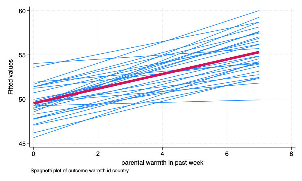 #### R
TipRandom Slopes and Random Intercepts
This spaghetti plot is illustrating the idea of random intercepts and random slopes. The multilevel model is estimating group specific regression lines, in this case country specific regression lines. Each country specific regression line has its own intercept and its own slope. The results presented in the multilevel model are the result of averaging these estimates into one overall estimate.
4.1.5 A Note On The Estimation of Random Effects
Procedures for estimating models with uncorrelated and correlated random effects are detailed below (StataCorp 2023; Bates et al. 2015).
| Software | Uncorrelated Random Effects | Correlated Random Effects |
|---|---|---|
| Stata | default | add option: , cov(uns) |
| R | separate random effects from grouping variable with || |
separate random effects from grouping variable with | |
All models in the examples below are run with uncorrelated random effects, but could just as easily be run with correlated random effects.
4.1.6 Unconditional Model
4.1.6.1 Model
mixed outcome || country: // unconditional modelPerforming EM optimization ...
Performing gradient-based optimization:
Iteration 0: Log likelihood = -9802.8371
Iteration 1: Log likelihood = -9802.8371
Computing standard errors ...
Mixed-effects ML regression Number of obs = 3,000
Group variable: country Number of groups = 30
Obs per group:
min = 100
avg = 100.0
max = 100
Wald chi2(0) = .
Log likelihood = -9802.8371 Prob > chi2 = .
------------------------------------------------------------------------------
outcome | Coefficient Std. err. z P>|z| [95% conf. interval]
-------------+----------------------------------------------------------------
_cons | 52.43327 .3451217 151.93 0.000 51.75685 53.1097
------------------------------------------------------------------------------
------------------------------------------------------------------------------
Random-effects parameters | Estimate Std. err. [95% conf. interval]
-----------------------------+------------------------------------------------
country: Identity |
var(_cons) | 3.178658 .9226736 1.799552 5.614658
-----------------------------+------------------------------------------------
var(Residual) | 39.46106 1.024013 37.50421 41.52
------------------------------------------------------------------------------
LR test vs. linear model: chibar2(01) = 166.31 Prob >= chibar2 = 0.00004.1.6.2 ICC
estat iccIntraclass correlation
------------------------------------------------------------------------------
Level | ICC Std. err. [95% conf. interval]
-----------------------------+------------------------------------------------
country | .0745469 .0201254 .0434963 .1248696
------------------------------------------------------------------------------4.1.7 Conditional Model
mixed outcome warmth physical_punishment identity i.intervention HDI || country: warmth // multilevel model

est store crosssectional // store estimates
Performing EM optimization ...
Performing gradient-based optimization:
Iteration 0: Log likelihood = -9626.6279
Iteration 1: Log likelihood = -9626.607
Iteration 2: Log likelihood = -9626.607
Computing standard errors ...
Mixed-effects ML regression Number of obs = 3,000
Group variable: country Number of groups = 30
Obs per group:
min = 100
avg = 100.0
max = 100
Wald chi2(5) = 334.14
Log likelihood = -9626.607 Prob > chi2 = 0.0000
-------------------------------------------------------------------------------
outcome | Coefficient Std. err. z P>|z| [95% conf. interval]
--------------+----------------------------------------------------------------
warmth | .8345368 .0637213 13.10 0.000 .7096453 .9594282
physical_pu~t | -.9916657 .0797906 -12.43 0.000 -1.148052 -.8352791
identity | -.3004767 .2170295 -1.38 0.166 -.7258466 .1248933
1.intervent~n | .6396427 .2174519 2.94 0.003 .2134448 1.065841
HDI | -.003228 .0199257 -0.16 0.871 -.0422817 .0358256
_cons | 51.99991 1.371257 37.92 0.000 49.3123 54.68753
-------------------------------------------------------------------------------
------------------------------------------------------------------------------
Random-effects parameters | Estimate Std. err. [95% conf. interval]
-----------------------------+------------------------------------------------
country: Independent |
var(warmth) | .0227504 .0257784 .0024689 .2096436
var(_cons) | 2.963975 .9737646 1.556777 5.643163
-----------------------------+------------------------------------------------
var(Residual) | 34.97499 .9097109 33.23668 36.80422
------------------------------------------------------------------------------
LR test vs. linear model: chi2(2) = 205.74 Prob > chi2 = 0.0000
Note: LR test is conservative and provided only for reference.library(lme4)
fit1 <- lmer(outcome ~ warmth + physical_punishment +
identity + intervention + HDI +
(1 + warmth || country),
data = simulated_multilevel_data)
summary(fit1)Linear mixed model fit by REML ['lmerMod']
Formula: outcome ~ warmth + physical_punishment + identity + intervention +
HDI + ((1 | country) + (0 + warmth | country))
Data: simulated_multilevel_data
REML criterion at convergence: 19268.8
Scaled residuals:
Min 1Q Median 3Q Max
-3.9774 -0.6563 0.0187 0.6645 3.6730
Random effects:
Groups Name Variance Std.Dev.
country (Intercept) 3.19056 1.786
country.1 warmth 0.02465 0.157
Residual 35.01782 5.918
Number of obs: 3000, groups: country, 30
Fixed effects:
Estimate Std. Error t value
(Intercept) 52.011364 1.414872 36.760
warmth 0.834562 0.064252 12.989
physical_punishment -0.991892 0.079845 -12.423
identity -0.300350 0.217179 -1.383
intervention 0.639059 0.217603 2.937
HDI -0.003395 0.020596 -0.165
Correlation of Fixed Effects:
(Intr) warmth physc_ idntty intrvn
warmth -0.124
physcl_pnsh -0.149 -0.003
identity -0.072 -0.012 -0.003
interventin -0.082 0.034 0.022 -0.018
HDI -0.943 -0.006 0.009 -0.001 0.0004.2 Longitudinal Model
4.2.1 Get Data
use "simulated_multilevel_longitudinal_data.dta", clear4.2.2 The Equation
\[\begin{aligned} \text{outcome}_{ij} = \beta_0 + \beta_1 \text{parental warmth} + \beta_2 \text{physical punishment} + \beta_3 \text{time} + \\ \beta_4 \text{identity}_2 + \beta_5 \text{intervention} + \beta_5 HDI + \\ u_{0j} + u_{1j} \times \text{parental warmth} + \\ v_{0i} + v_{1i} \times t + e_{ij} \end{aligned} \tag{4.2}\]
4.2.3 Descriptive Statistics
summarize // descriptive statistics Variable | Obs Mean Std. dev. Min Max
-------------+---------------------------------------------------------
country | 9,000 15.5 8.655922 1 30
HDI | 9,000 64.76667 17.2437 33 87
family | 9,000 50.5 28.86767 1 100
id | 0
identity | 9,000 .4976667 .5000223 0 1
-------------+---------------------------------------------------------
intervention | 9,000 .4843333 .4997823 0 1
t | 9,000 2 .8165419 1 3
physical_p~t | 9,000 2.485333 1.373639 0 5
warmth | 9,000 3.514222 1.8839 0 7
outcome | 9,000 53.37768 6.572285 29.60798 79.021994.2.4 Alternate Plot
encode id, generate(idNUMERIC) // numeric version of id
* spagplot outcome t if idNUMERIC <= 10, id(idNUMERIC) scheme(stcolor)
twoway (lfit outcome t) (scatter outcome t) if idNUMERIC <= 10, by(idNUMERIC) scheme(stcolor)
graph export spagplot2.png, width(1000) replace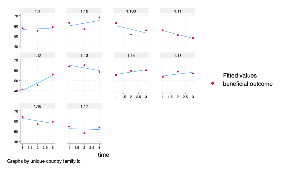 #### R
4.2.5 Unconditional Model
4.2.5.1 Model
mixed outcome || country: || id: // unconditional model4.2.5.2 ICC
estat iccIntraclass correlation
------------------------------------------------------------------------------
Level | ICC Std. err. [95% conf. interval]
-----------------------------+------------------------------------------------
country | .0748336 .0190847 .0450028 .1219141
id|country | .3462837 .017146 .3134867 .3806097
------------------------------------------------------------------------------4.2.6 Conditional Model
mixed outcome t warmth physical_punishment i.identity i.intervention HDI || country: warmth || id: t // multilevel model

est store longitudinal // store estimates
Performing EM optimization ...
Performing gradient-based optimization:
Iteration 0: Log likelihood = -28523.49
Iteration 1: Log likelihood = -28499.973
Iteration 2: Log likelihood = -28499.736
Iteration 3: Log likelihood = -28499.604
Iteration 4: Log likelihood = -28499.603
Computing standard errors ...
Mixed-effects ML regression Number of obs = 9,000
Grouping information
-------------------------------------------------------------
| No. of Observations per group
Group variable | groups Minimum Average Maximum
----------------+--------------------------------------------
country | 30 300 300.0 300
id | 3,000 3 3.0 3
-------------------------------------------------------------
Wald chi2(6) = 1096.15
Log likelihood = -28499.603 Prob > chi2 = 0.0000
-------------------------------------------------------------------------------
outcome | Coefficient Std. err. z P>|z| [95% conf. interval]
--------------+----------------------------------------------------------------
t | .943864 .0658716 14.33 0.000 .814758 1.07297
warmth | .913496 .0423731 21.56 0.000 .8304462 .9965457
physical_pu~t | -1.007897 .0497622 -20.25 0.000 -1.105429 -.9103647
1.identity | -.1276926 .1515835 -0.84 0.400 -.4247909 .1694056
1.intervent~n | .8589966 .1519094 5.65 0.000 .5612596 1.156734
HDI | -.0005657 .0196437 -0.03 0.977 -.0390666 .0379352
_cons | 50.46724 1.338319 37.71 0.000 47.84418 53.09029
-------------------------------------------------------------------------------
------------------------------------------------------------------------------
Random-effects parameters | Estimate Std. err. [95% conf. interval]
-----------------------------+------------------------------------------------
country: Independent |
var(warmth) | .0107584 .0127845 .0010477 .1104715
var(_cons) | 3.167089 .9146769 1.798157 5.578187
-----------------------------+------------------------------------------------
id: Independent |
var(t) | 2.01e-09 4.14e-07 3.2e-185 1.3e+167
var(_cons) | 8.387272 .4724189 7.510628 9.36624
-----------------------------+------------------------------------------------
var(Residual) | 26.02734 .4753701 25.11211 26.97592
------------------------------------------------------------------------------
LR test vs. linear model: chi2(4) = 1247.03 Prob > chi2 = 0.0000
Note: LR test is conservative and provided only for reference.4.2.7 Nice Table of Results
etable, estimates(crosssectional longitudinal) ///
showstars showstarsnote /// show stars and note
column(estimate) // column is modelname
crosssectional longitudinal
----------------------------------------------------------------
parental warmth in past week 0.835 ** 0.913 **
(0.064) (0.042)
physical punishment in past week -0.992 ** -1.008 **
(0.080) (0.050)
hypothetical identity group variable -0.300
(0.217)
recieved intervention
1 0.640 ** 0.859 **
(0.217) (0.152)
Human Development Index -0.003 -0.001
(0.020) (0.020)
time 0.944 **
(0.066)
hypothetical identity group variable
1 -0.128
(0.152)
Intercept 52.000 ** 50.467 **
(1.371) (1.338)
var(warmth) 0.023 0.011
(0.026) (0.013)
var(_cons) 2.964 3.167
(0.974) (0.915)
var(e) 34.975 26.027
(0.910) (0.475)
var(_cons) 8.387
(0.472)
var(t) 0.000
(0.000)
Number of observations 3000 9000
----------------------------------------------------------------
** p<.01, * p<.05