Why Multilevel Models Are Good Models For Longitudinal Data

Multilevel Models Offer An Incredibly Flexible Treatment of Time and Time Varying Processes and Covariates

1 Key Idea

Multilevel Models are Useful for Complicated Longitudinal Data and Research Designs

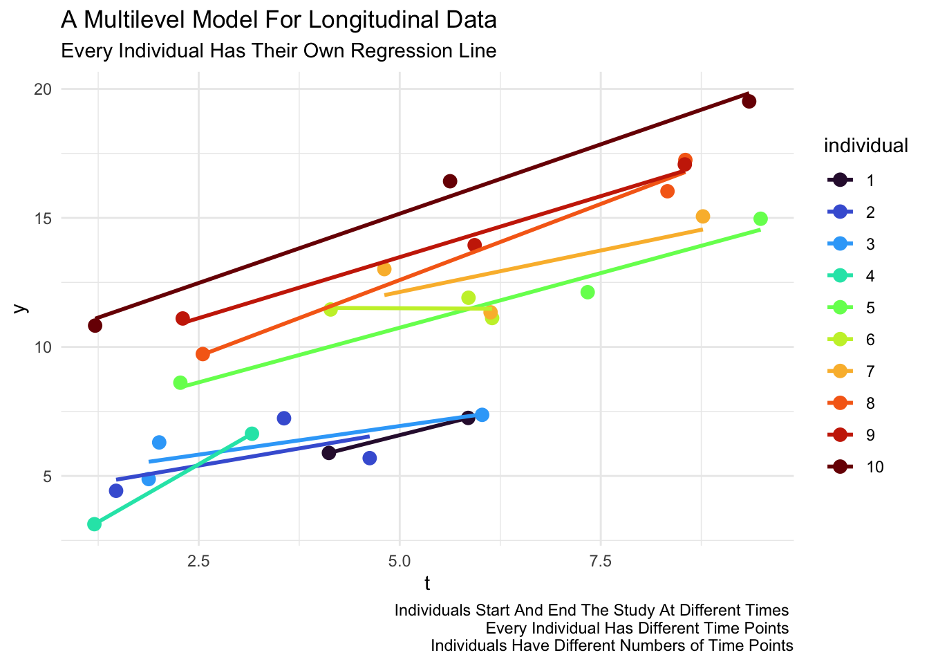
Multilevel models are uniquely suited for complicated longitudinal data and research designs. Among other advantages, multilevel models are able to easily accommodate designs where individuals are observed at different times and different numbers of times.¹

2 Visually

Figure 1: A Multilevel Model For Longitudinal Data

3 Data Structures

Multilevel models for longitudinal data prefer data in long format.

Table 1: Data in WIDE format

id	x1	x2	x3	y1	y2	y3
1
2
3

Table 2: Data in LONG format

id	t	x	y
1	1
1	2
1	3
2	1
2	2
2	3
3	1
3	2
3	3

4 Equation

\[y_{it} = \beta_0 + \beta_1 t_{it} + \beta_2 x_{it} + u_{0i} + e_{it} \tag{1}\]

Person-Observations

Every row is a person-observation (person i observed at time t). Every person has multiple rows.

5 Advantages of the Multilevel Model for Longitudinal Data

1. Using the algebra in Equation 1, these models can easily accommodate both time varying and time invariant coefficients (Hox, 2010; Hox et al., 2018; Rabe-Hesketh & Skrondal, 2022; Raudenbush & Bryk, 2002; Singer & Willett, 2003).
2. There is no multicollinearity issue with multiple \(\beta\) coefficients for multiple waves of data. By inspection of Equation 1, we see that there is only a single \(\beta\) coefficient for each variable, \(\therefore\) no multicollinearity problem.
3. Unbalanced data is less of a problem, the data structure and estimation are robust to these possibilities (Raudenbush, 1995; Raudenbush & Bryk, 2002; Singer & Willett, 2003).
4. Missing data is less of a problem (assuming MCAR). When a person observation is missing, that person simply has fewer rows of data (Hox, 2010; Luke, 2004; Rabe-Hesketh & Skrondal, 2022; Raudenbush, 1995; Raudenbush & Bryk, 2002). But all rows of data are “matched” to the same person by \(i\).
5. We have an explicit function of time \(\beta_1 t\), and could treat time more flexibly, by creating a polynomial function of time e.g. by adding \(\beta_2 t^2\), etc. (Raudenbush & Bryk, 2002; Singer & Willett, 2003). (We could even substitute \(\beta \ln(t)\).)
6. Again, by inspection of Equation 1, we see that multiple or many time-points are not a problem. We would use the same algebra for 2 time points or for 10,000 time points. (Helpful when we start to think about intensive longitudinal data e.g. George Holden’s recording study).
7. We are measuring exactly the time at which events take place for each individual (Luke, 2004; Singer & Willett, 2003). Not simply saying Wave 1, Wave 2, Wave 3, etc…
8. Unequally spaced time points are not a problem (Raudenbush, 1995). Every individual could have a completely different set of time points and even a completely different number of time points (Hox, 2010; Hox et al., 2018; Luke, 2004; Singer & Willett, 2003).

Caution

We do need to think carefully about what is the appropriate variable for time. Is it the variable we used to reshape the data–often wave–or some other more appropriate metric, like age or time in study (Singer & Willett, 2003)?

6 References

Hox, J. (2010). Multilevel analysis: Techniques and applications (2nd ed.). Routledge.

Hox, J., Moerbeek, M., & van de Schoot, R. (2018). Multilevel analysis: Techniques and applications (Third edition.). Routledge, Taylor & Francis Group,.

Luke, D. (2004). Multilevel modeling. SAGE Publications, Inc. https://doi.org/10.4135/9781412985147

Rabe-Hesketh, S., & Skrondal, A. (2022). Multilevel and longitudinal modeling using stata. In Stata Press (4th ed.). Stata Press.

Raudenbush, S. W. (1995). Hierarchical linear models to study the effects of social context on development. In J. M. Gottman (Ed.), The analysis of change (pp. 165–199). Lawrence Erlbaum Associates.

Raudenbush, S. W., & Bryk, A. S. (2002). Hierarchical linear models: Applications and data analysis methods. Sage Publications.

Singer, J. D., & Willett, J. B. (2003). Applied longitudinal data analysis : Modeling change and event occurrence. Oxford University Press.

Footnotes

1. Many, if not most, of the advantages listed in this handout will also apply to any approach using long data.