| country | HDI | family | id | identity | intervention | t |
|---|---|---|---|---|---|---|
| 1 | 69 | 1 | 1.1 | 2 | 1 | 1 |
| 1 | 69 | 1 | 1.1 | 2 | 1 | 2 |
| 1 | 69 | 1 | 1.1 | 2 | 1 | 3 |
| 1 | 69 | 2 | 1.2 | 2 | 2 | 1 |
| 1 | 69 | 2 | 1.2 | 2 | 2 | 2 |
| 1 | 69 | 2 | 1.2 | 2 | 2 | 3 |
| physical_punishment | warmth | outcome |
|---|---|---|
| 3 | 3 | 58.47 |
| 3 | 4 | 56.06 |
| 1 | 2 | 59.77 |
| 2 | 1 | 51.1 |
| 3 | 0 | 54.31 |
| 3 | 1 | 50.79 |
“Mathematics is the art of giving the same name to different things.” (Poincare, 1908)
Counter-intuitively, and surprisingly, the mathematics of estimating models with cross-sectional clustered data easily generalizes to longitudinal data. In cross sectional clustered data, we imagine individuals or families clustered in neighborhoods, schools, or countries.
| Level | Example(s) |
|---|---|
| 1 | Individuals or Families |
| 2 | Schools |
| Neighborhoods | |
| Countries |
In longitudinal data, we consider the first level to be that of time points, or study waves, which we sometimes call the person-observation.1 The second level is then the individual or family.
| Level | Example(s) |
|---|---|
| 1 | Timepoints |
| 2 | Individuals or Families |
While it is less common, we could then easily add additional clustering to this longitudinal model, for example, clustering of individuals or families inside social units.
| Level | Example(s) |
|---|---|
| 1 | Timepoints |
| 2 | Individuals or Families |
| 3 | Schools |
| Neighborhoods | |
| Countries |
Multilevel data suitable for longitudinal analysis has multiple rows of data per individual or family. Put another way, every row of data is a person-timepoint.
This method of organizing data is known as the long format. Another way of organizing longitudinal data–which I do not discuss in detail here–is the wide format in which every individual or family has only a single row of data. In wide data, the different timepoints are in different columns of data. I do discuss reshaping data from wide to long, and vice versa, in the Appendix.
| id | t | x |
|---|---|---|
| 1 | 1 | 10 |
| 1 | 2 | 20 |
| 1 | 3 | 30 |
| 2 | 1 | 20 |
| 2 | 2 | 30 |
| 2 | 3 | 40 |
| id | x1 | x2 | x3 |
|---|---|---|---|
| 1 | 10 | 20 | 30 |
| 2 | 20 | 30 | 40 |
For the discussion below, I use a longitudinal version of the simulated data that has multiple rows of data per family.
| country | HDI | family | id | identity | intervention | t |
|---|---|---|---|---|---|---|
| 1 | 69 | 1 | 1.1 | 2 | 1 | 1 |
| 1 | 69 | 1 | 1.1 | 2 | 1 | 2 |
| 1 | 69 | 1 | 1.1 | 2 | 1 | 3 |
| 1 | 69 | 2 | 1.2 | 2 | 2 | 1 |
| 1 | 69 | 2 | 1.2 | 2 | 2 | 2 |
| 1 | 69 | 2 | 1.2 | 2 | 2 | 3 |
| physical_punishment | warmth | outcome |
|---|---|---|
| 3 | 3 | 58.47 |
| 3 | 4 | 56.06 |
| 1 | 2 | 59.77 |
| 2 | 1 | 51.1 |
| 3 | 0 | 54.31 |
| 3 | 1 | 50.79 |
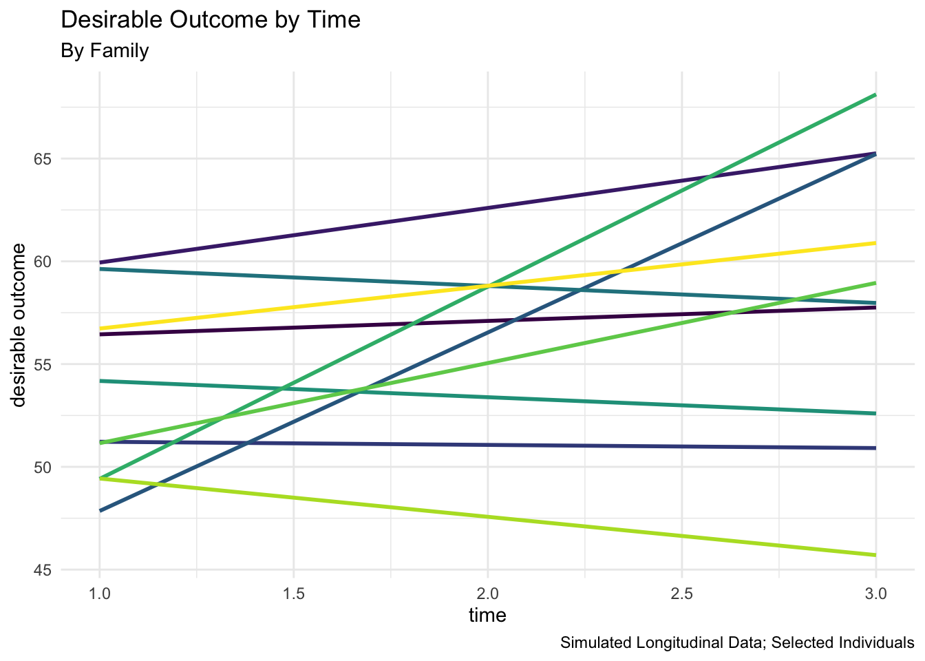
Since I will be discussing the estimation of a longitudinal model, it is often useful to graph the outcome variable against time.
When data are in long format, the following equation is applicable. Observe that the model below is a three level model where timepoints are nested inside families which in turn are nested inside countries. A simpler two level model with timepoints nested inside families would also be possible to estimate.
\[\text{outcome}_{itj} = \beta_0 + \beta_1 \text{parental warmth}_{itj} + \beta_2 \text{physical punishment}_{itj} + \beta_3 \text{time}_{itj} \ + \tag{6.1}\]
\[\beta_4 \text{identity}_{itj} + \beta_5 \text{intervention}_{itj} + \beta_6 \text{HDI}_{itj} +\]
\[u_{0j} + u_{1j} \times \text{parental warmth}_{itj} \ + \]
\[v_{0i} + v_{1i} \times \text{time}_{itj} + e_{itj}\] Here I include a random slope (\(u_{1j}\)) at the country level for parental warmth, as well as a random slope (\(v_{1i}\)) at the family level for time.
As before, the random slope for parental warmth, \(u_{1j} \times \text{parental warmth}_{ij}\) suggests allows us to estimate whether the relationship between parental warmth and the outcome varies across countries. The random slope for time, \(v_{1i} \times t\), allows us to estimate whether time trajectories (the slope for time) vary across families.
In longitudinal multilevel models, the variable for time assumes a special role as we are often visualizing a growth trajectory over the course of time.
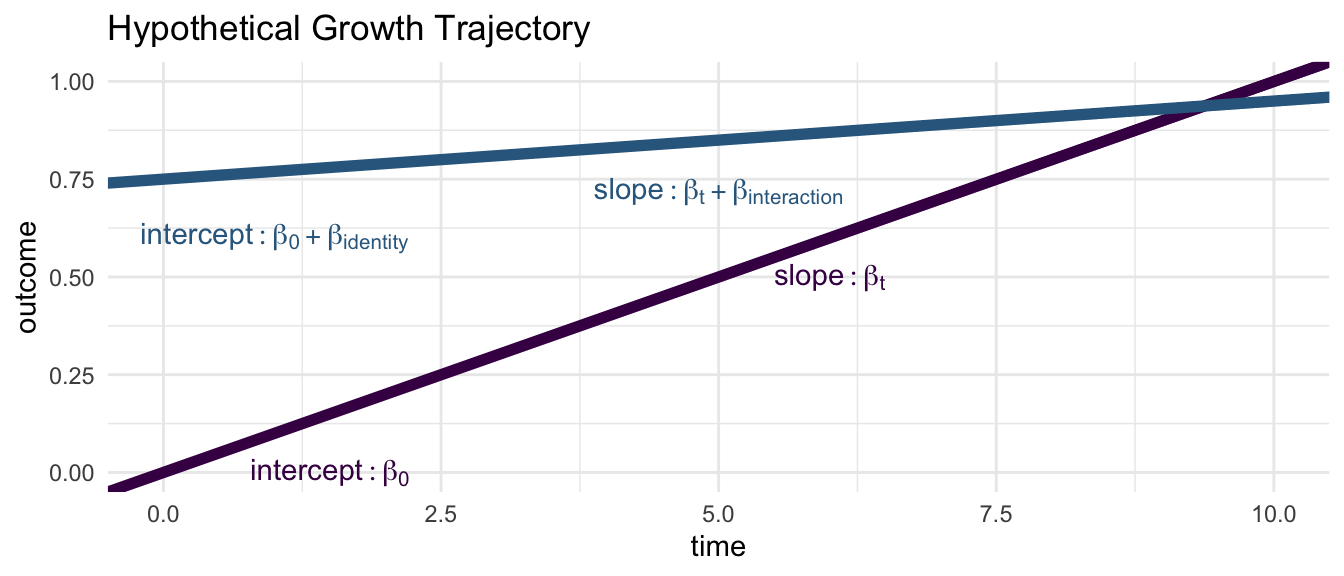
Imagine a model as follows where identity is a (1/0) variable for membership in one of two groups:
\[\text{outcome} = \beta_0 + \beta_t \text{time} + \beta_\text{identity} \text{identity} + \beta_\text{interaction} \text{identity} \times \text{time} + u_{0i} + e_{it}\] Then, each identity group has its own intercept and time trajectory:
| Group | Intercept | Slope (Time Trajectory) |
|---|---|---|
| 0 | \(\beta_0\) | \(\beta_t\) |
| 1 | \(\beta_0 + \beta_\text{identity}\) | \(\beta_t + \beta_\text{interaction}\) |
Thus, in longitudinal multilevel models, main effects modify the intercept of the time trajectory, while interactions with time, modify the slope of the time trajectory.
| 1 | ||
|---|---|---|
| t | 0.944 | ** |
| warmth | 0.913 | ** |
| physical_punishment | -1.008 | ** |
| identity | ||
| 2 | -0.128 | |
| intervention | ||
| 2 | 0.859 | ** |
| HDI | -0.001 | |
| _cons | 51.467 | ** |
| var(warmth) | 0.011 | |
| var(_cons) | 3.167 | |
| var(_cons) | 8.387 | |
| var(t) | 0.000 | |
| var(e) | 26.027 | |
| Number of observations | 9000 |
** p<.01, * p<.05
Examining the regression results, the results of the model suggest that child outcomes improve over time. Better child outcomes are again associated with parental warmth, and parental use of physical_punishment is associated with reduced child outcomes. identity is not associated with the outcome. However, the intervention is associated with increases in the outcome. HDI is again not associated with outcomes.
As discussed in Section 6.4, we will likely wish to model not only associations of other independent variables with the intercept of the time trajectory, but also associations of other independent variables with the slope of the time trajectory. Accordingly, we modify Equation 6.2 so that it includes these interactions. Below, I add the letter \(B\) to some \(\beta\) coefficients to denote that they are a second coefficient estimating the interaction of that variable with time.
\[\text{outcome}_{itj} = \beta_0 + \beta_1 \text{parental warmth}_{itj} + \beta_2 \text{physical punishment}_{itj} + \beta_3 \text{time}_{itj} \ + \tag{6.2}\]
\[\beta_{1B} \text{parental warmth}_{itj} \times \text{time}_{itj} + \beta_{2B} \text{physical punishment}_{itj} \times \text{time}_{itj} +\]
\[\beta_4 \text{identity}_{itj} + \beta_5 \text{intervention}_{itj} + \beta_6 \text{HDI}_{itj} +\]
\[\beta_{4B} \text{identity}_{itj} \times \text{time}_{itj} + \beta_{5B} \text{intervention}_{itj} \times \text{time}_{itj} + \beta_{6B} \text{HDI}_{itj} \times \text{time}_{itj} +\]
\[u_{0j} + u_{1j} \times \text{parental warmth}_{itj} \ + \]
\[v_{0i} + v_{1i} \times \text{time}_{itj} + e_{itj}\]
| 1 | ||
|---|---|---|
| t | 0.758 | * |
| warmth | 0.817 | ** |
| physical_punishment | -1.009 | ** |
| identity | ||
| 2 | -0.239 | |
| intervention | ||
| 2 | 0.661 | * |
| HDI | 0.001 | |
| t # warmth | 0.048 | |
| t # physical_punishment | 0.001 | |
| identity # t | ||
| 2 | 0.055 | |
| intervention # t | ||
| 2 | 0.099 | |
| t # HDI | -0.001 | |
| _cons | 51.836 | ** |
| var(warmth) | 0.011 | |
| var(_cons) | 3.170 | |
| var(_cons) | 8.392 | |
| var(t) | 0.000 | |
| var(e) | 26.016 | |
| Number of observations | 9000 |
** p<.01, * p<.05
Examining the regression results, the results of the model again suggest that child outcomes improve over time. Better child outcomes are again associated with parental warmth, and parental use of physical_punishment is associated with reduced child outcomes. identity is again not associated with outcomes, while participation in the intervention is associated with improvements in outcomes. HDI is again not associated with outcomes.
Examining the interaction terms, we find that none of these variables modify the time trajectory of the outcome.
When data are ordered by a time variable \(t\), it is possible that observations that are closer together in time will have a higher correlation than observations that are distant in time. In the simplest example, \(e_{i, t=k}\) may be correlated with \(e_{i, t=k-1}\). This phenomenon is known as autocorrelation. As Hooper (2022) would suggest, it may make sense to assume that the correlation between observations “decays with increasing separation in time”.
Most software programs for multilevel modeling allow one to incorporate measures of autocorrelation so that, e.g., \(e_{i,t=3}\) is allowed to be correlated with \(e_{i,t=2}\), which in turn can be correlated with \(e_{i,t=1}\). More complex autocorrelation structures are usually also possible (StataCorp, 2021a).
Causal reasoning is sometimes considered to be a statistical–or even overly technical–concern. Arguably, however, whenever one is using research to make recommendations about interventions, or treatments, or policies, one is engaging in some form of causal reasoning (Duncan & Gibson-Davis, 2006).
If one is saying that implementing x would result in beneficial changes in y, one is arguing–at least implicitly–that x is one of the causes of y.
It then behooves one to be explicit about this chain of causal reasoning. For example, to continue one of the substantive examples of this book, if one is going to argue for programs, interventions, or treatments that promote parental warmth, or that discourage parental use of physical punishment with the aim of improving children’s mental health, one must be at least reasonably sure that parental warmth and physical punishment are causes of children’s mental health.
In a statement salient for social research, Duncan & Gibson-Davis (2006) point out the logical inconsistency of writing that does not rigorously address causal processes, but then goes on to suggest interventions or treatment or policies:
“Developmental studies are usually careful to point out when their data do not come from a randomized experiment. As with much of the nonexperimental literature in developmental psychology, most of the articles then go on to assert that, as a consequence, it is impossible to draw causal inferences from the analysis. Indeed, much of their language describing results is couched in terms of ‘associations’ between child care quality and child outcomes. It is not uncommon, however, to see these papers make explicit statements about effects, and others draw explicit policy conclusions. For instance, NICHD (1997, 876) stated, ‘The interaction analyses provided evidence that high-quality child care served a compensatory function for children whose maternal care was lacking.’ On the policy side, NICHD (2002c, 199) asserted, ‘These findings provide empirical support for policies that improve state regulations for caregiver training and child-staff ratios.’”
“One cannot have it both ways. Studies that do not aspire to causal analysis should make no claim whatsoever about effects and draw no policy conclusions. At the same time, it would be a terrible waste of resources to conduct expensive longitudinal studies without attempting to use them for causal modeling.”
Randomized studies provide the best evidence about internal validity and causal relationships. However, randomized studies have certain important limitations (Diener et al., 2022). First of all–especially in a study with a smaller sample–randomization may not always be perfect, and the control and treatment groups may not be statistically equivalent. Secondly, because randomized studies are costly to conduct, they may have small samples and may be statistically underpowered. Smaller samples and underpowered studies are more likely to generate false positive results than larger samples (Button et al., 2013) 2. Further, and importantly, because of ethical concerns some studies can not be conducted with randomization (Diener et al., 2022). For example, in the study of parenting and child development, children cannot ethically be assigned to parents with different styles of parenting and followed over the long term (Heilmann et al., 2021). Finally, and crucially, because of their often small samples, and their often rigorous exclusion criteria, randomized studies may have high internal validity, but much lower external validity, or generalization to larger populations (Diener et al., 2022). This issue of generalizability becomes increasingly salient, when we are reminded of the fact that so little social and psychological research has been conducted outside of North American contexts (Draper et al., 2022; Henrich et al., 2010). Thus, methods that provide rigorous causal estimation with observational methods are necessary (Diener et al., 2022).
Because of the assumed superiority of studies that employ randomization, it is sometimes maintained that correlation is not causation and that studies that do not make use of randomization are only observational and correlational, and that results from observational studies cannot be used to support causal conclusions. However, in an important review (Waddington et al., 2022) suggested that studies using appropriately quantitative methods can provide causally robust conclusions. Heilmann et al. (2021) make a similar assertion with specific regard to studies of physical punishment and child outcomes, arguing that observational studies that make use of appropriately advanced quantitative methods can make causally robust conclusions about the effects of physical discipline.
It is necessary to make use of broadly representative observational data sets, and appropriately sophisticated quantitative methods, to make causally robust conclusions from observational data that are applicable across diverse populations.
For x to be a cause of y, one needs the following 3 things to be true (Holland, 1986).
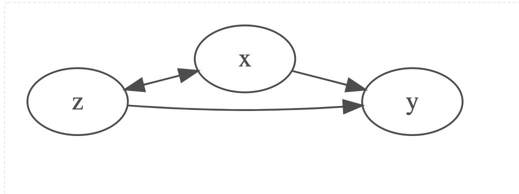
If z is omitted from the regression model, then the estimates for \(x \rightarrow y\) (i.e. \(\beta_{x \rightarrow y}\)) will be biased. In a common scenario, \(\beta_{x \rightarrow y}\) may be an over-estimate of the effect, and statistical significance of \(\beta_{x \rightarrow y}\) may represent a false positive.
It is likely useful to restate the above abstract statements in terms of the substantive issues that I have been considering so far in this book.
For parenting to be a cause of child outcomes, one needs the following 3 things to be true (Holland, 1986).
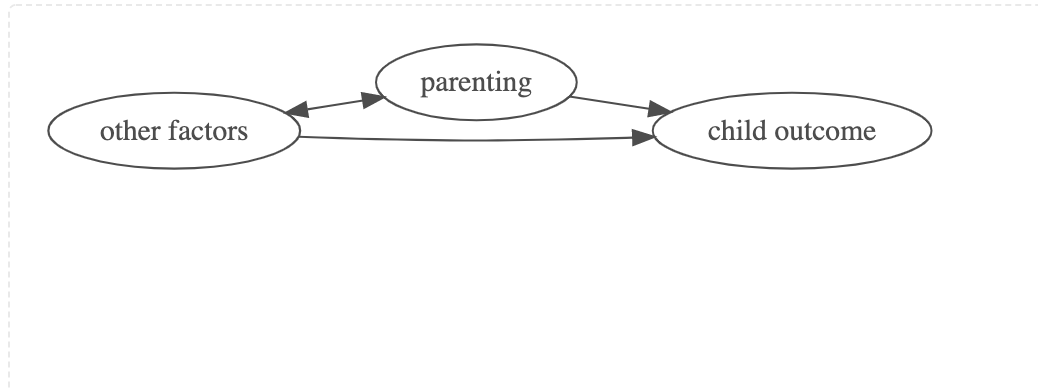
If other factors are omitted from the regression model, then the estimates for \(\text{parenting} \rightarrow \text{child outcome}\) (i.e. \(\beta_{\text{parenting} \rightarrow \text{child outcome}}\)) will be biased. In a common scenario, \(\beta_{\text{parenting} \rightarrow \text{child outcome}}\) may be an over-estimate of the effect, and statistical significance of \(\beta_{\text{parenting} \rightarrow \text{child outcome}}\) may represent a false positive.
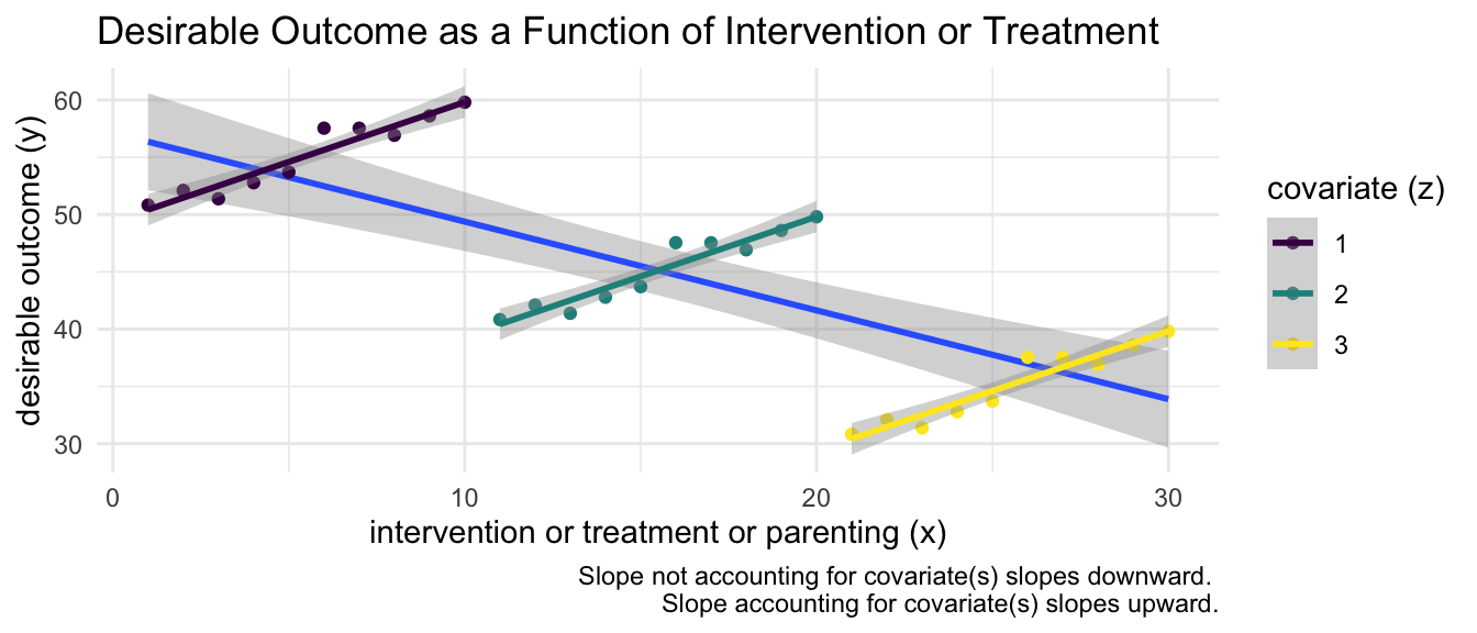
Earlier, in Section 5.2, I referred to the idea of multilevel structure wherein failure to account for the clustering of data–omission of \(u_0\) from the equation being estimated–may lead to incorrect conclusions. A closely related phenomenon is that of Simpson’s Paradox (Simpson, 1951) wherein omission of a relevant covariate (e.g. \(z_{it}\) such as SES, community characteristics, country level characteristics) may also lead to dramatically incorrect results.
Statistically, we imagine a situation where the true model is:
\[\text{child outcome}_{it} = \beta_0 + \beta_1 \text{parenting}_{it} +\]
\[\beta_2 \text{individual or family or community or country characteristic}_{it} + \] \[u_{0i} + e_{it}\]
If individual or family or community or country characteristics in fact influence outcome, but are not included in the statistical model, perhaps because they are not measured in the data, then the estimate of \(\beta_1\) for parenting will be biased. See Figure 6.5 for an illustration. When possible confounders are measured, we can include those variables in the statistical model. When possible confounders are unmeasured, we need to try to use methods that capture those unmeasured confounders.
For purposes of explication of ideas about causal estimation, in this section, I imagine a simpler equation where I am only considering the clustering of person timepoints within individual people, and ignoring for the moment–again for the sake of exposition–the clustering of individuals within countries.
After explication and comprehension of this model, however, it is a simple matter to add back in the random effects for country level clustering.
The appropriate multilevel model is below.
\[\text{outcome}_{it} = \beta_0 + \beta_1 \text{parental warmth}_{it} + \beta_2 \text{physical punishment}_{it} + \beta_3 \text{time}_{it} \ + \tag{6.3}\]
\[\beta_4 \text{identity}_{it} + \beta_5 \text{intervention}_{it} + \beta_6 \text{HDI}_{it} \ +\]
\[v_{0i} + e_{it}\]
Note that in Equation 6.3, if one were estimating a multilevel model, one would consider the \(v_{0i}\) to be a randomly varying parameter with a mean of 0, and a variance of \(\sigma^2(v_{0i})\).
I can use the same equation:
\[\text{outcome}_{it} = \beta_0 + \beta_1 \text{parental warmth}_{it} + \beta_2 \text{physical punishment}_{it} + \beta_3 \text{time}_{it} \ + \tag{6.4}\]
\[\beta_4 \text{identity}_{it} + \beta_5 \text{intervention}_{it} + \beta_6 \text{HDI}_{it} \ +\]
\[v_{0i} + e_{it}\]
However, in Equation 6.4, I now consider the \(v_{0i}\) to be estimable for each individual \(i\) in the data. In effect, the \(v_{0i}\) become a unique indicator variable for each individual in the data set. This is known as a fixed effects regression model.
Recall the discussion in Section 5.6. In essence, in the fixed effects regression model, I am only making use of the variation within individuals, and not making use of the variation between individuals.
Details are provided in Allison (2009) and Wooldridge (2010). StataCorp (2021b) provides an exceptionally clear explication of the core idea of fixed effects regression. The essential idea is that the fixed effects model provides statistical control for all time invariant characteristics of study participants, such as–as is often the case in many data sets–their racial or ethnic identity, their neighborhood of residence, or other characteristics which by definition are time invariant, such as the region of the country or city in which a respondent was born. Importantly, (Ma et al., 2018) note that:
“Another potential omitted variable is that of genetic predisposition, in that observed neighborhood effects on child outcomes are possibly attributable to a genetic heritage shared by parents and their child (Caspi et al., 2000).”
Such genetic heritage could be considered to be a time invariant variable that, while unobserved, would be controlled for by a fixed effects regression.
Thus, by ruling out many potential confounds, fixed effects regression methods provide much more causally robust analyses, specifically because they control for many more possible confounding variables than do standard regression methods, including multilevel models, which are only able to control for the variables that are measured in the study and that are included within the regression model.
However, a disadvantage of the fixed effects approach is that this approach can not provide estimates for any time invariant characteristic of study participants. Indeed, if one includes time invariant variables into a fixed effects regression, they are automatically dropped from the regression results as can be seen in the regression table below.
| MLM | FE | |||
|---|---|---|---|---|
| t | 0.943 | ** | 0.944 | ** |
| warmth | 0.913 | ** | 0.916 | ** |
| physical_punishment | -0.982 | ** | -1.094 | ** |
| identity | ||||
| 2 | -0.116 | |||
| intervention | ||||
| 2 | 0.886 | ** | ||
| HDI | 0.001 | |||
| _cons | 51.298 | ** | 51.988 | ** |
| var(_cons) | 11.831 | |||
| var(e) | 26.033 | |||
| Number of observations | 9000 | 9000 |
** p<.01, * p<.05
In comparing the multilevel model and the fixed effects regression, we note a few salient difference. First, the fixed effects are similar to the multilevel model coefficients. (Most often, the fixed effect regression coefficients are attenuated versions of the multilevel model coefficients, but not always.) The fixed effects regression coefficients for variables that have some variation over time, provide estimates that control for all time invariant variables in the model.
Second, estimates for any quantities that do not vary over time, in this case, group membership, and HDI, are not available from the fixed effects regression.
When we are studying families, e.g. a parent-child pair, it might be more appropriate to call each row of data a family-observation, but the term person-observation is more commonly used.↩︎
See https://agrogan.shinyapps.io/Thinking-Through-Bayes/ for a demonstration of this idea from a Bayesian perspective.↩︎
The correlated random effects model can also be applied cross-sectionally, but the model is much easier to explicate in the longitudinal context.↩︎