Show the code
library(rnaturalearth) # natural earth data

library(ggplot2) # beautiful maps

library(dplyr) # data wrangling

library(sf) # simple (spatial) features

library(cartogram) # cartograms!cartogramA cartogram is a map where the areas of different regions are distorted (increased in size; decreased in size) by the value of some quantitative variable.
library(rnaturalearth) # natural earth data
library(ggplot2) # beautiful maps
library(dplyr) # data wrangling
library(sf) # simple (spatial) features
library(cartogram) # cartograms!options(scipen = 999) # high 'penalty' for scientific notationrnaturalearthmapdata <- ne_countries(scale = "medium", # medium scale
returnclass = "sf") # as sf objectWe make a basic map, reading it into an object called mymap. We then replay mymap.
mymap <- ggplot(mapdata) + # the data I am mapping
  geom_sf() # the geometry I am using

mymap # replay my map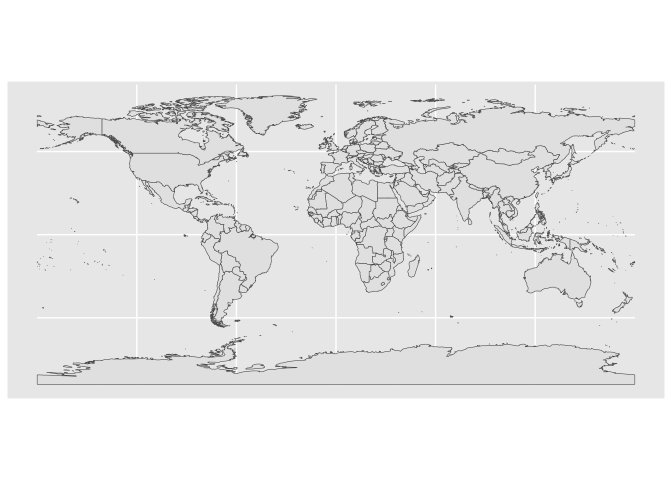
cartogram requires projected data (Chapter 5), so we need to project the data with st_transform. A number of projections, including the Mercator and Mollweide projections are possibilities. You may need to experiment with a number of projections to see which ones work best in any particular cartogram.
mapdata_proj <- st_transform(mapdata,
                             3857) # Mercator

# mapdata_proj <- st_transform(mapdata,
# crs = "+proj=moll") # Mollweideggplot(mapdata_proj) +
geom_sf() # plot projected data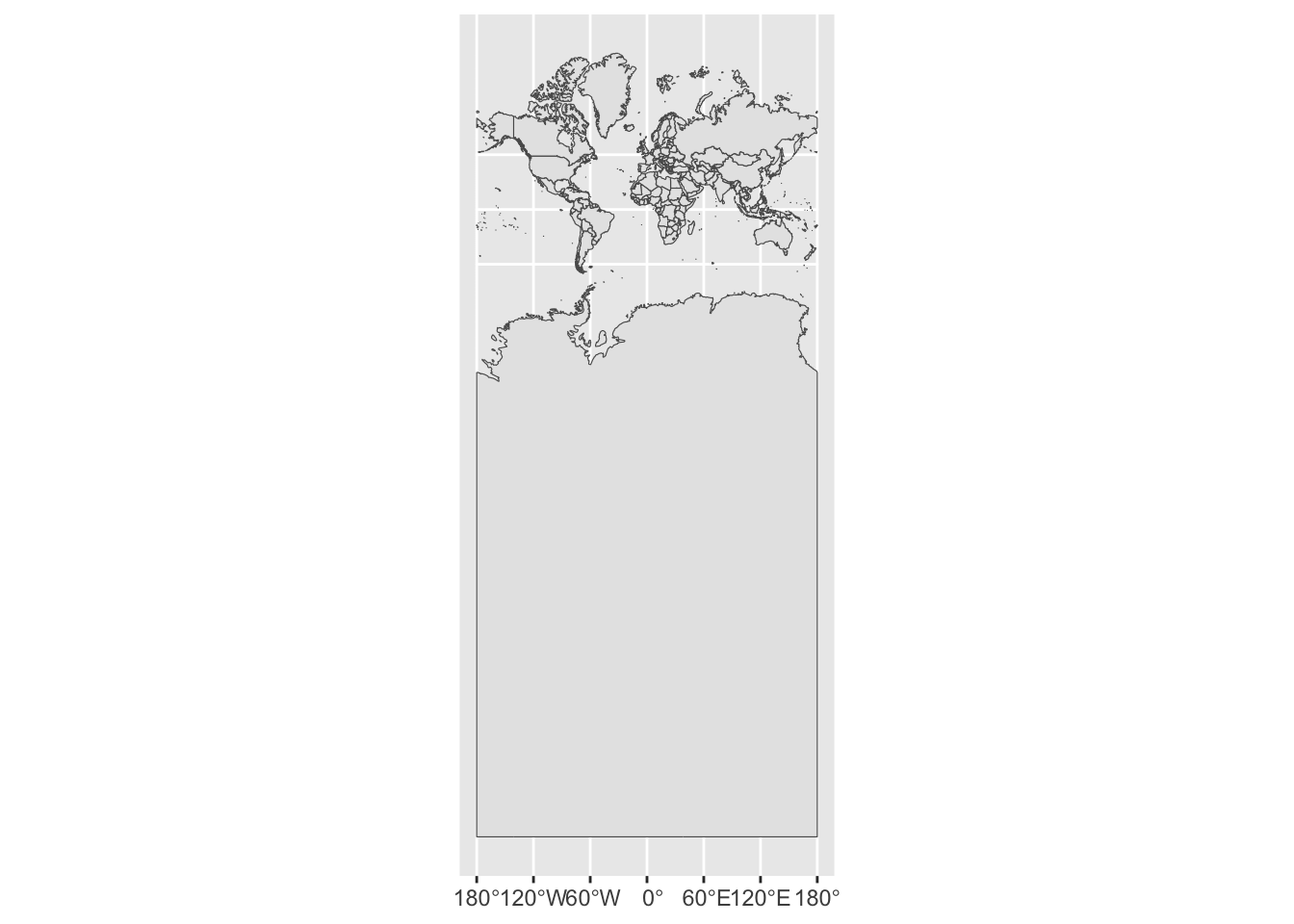
In some projections, especially the Mercator projection, Antarctica looks strange.
The key is to run this dplyr code to remove Antarctica.
mapdata_proj <- mapdata_proj %>%
dplyr::filter(! continent == "Antarctica")
ggplot(mapdata_proj) +
  geom_sf() # plot projected data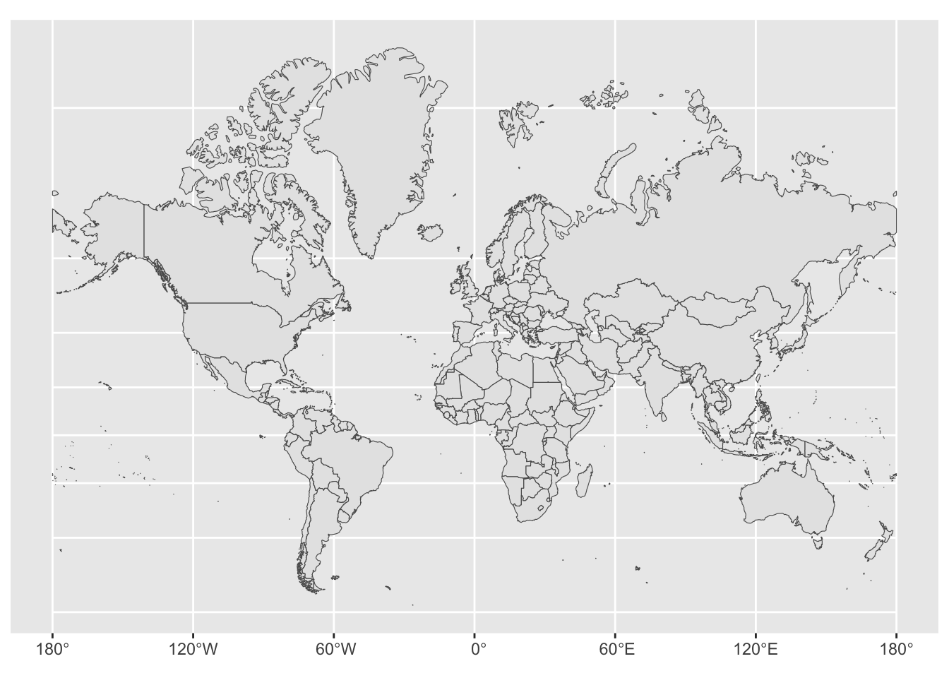
Each iteration takes a LONG time. Fewer iterations help the time, but each iteration contributes to the distortion, and makes a more cartogram-like cartogram. Because this is the most time intensive step, I time the creation of the cartogram with Sys.time.
start_time <- Sys.time() # time this step

mapdata_cartogram <- cartogram_cont(mapdata_proj,
                                  "pop_est",
                                  itermax = 7)
Warning in cartogram_cont.sf(mapdata_proj, "pop_est", itermax = 7): NA not
allowed in weight vector. Features will be removed from Shape.end_time <- Sys.time()
end_time - start_timeTime difference of 1.750577 minsggplot(mapdata_cartogram) +
geom_sf()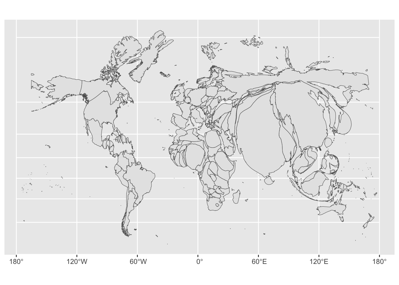
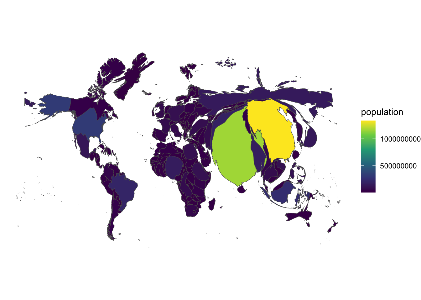
fill Colorggplot(mapdata_cartogram) +
geom_sf(aes(fill = pop_est)) + # fill is population estimate
theme_void()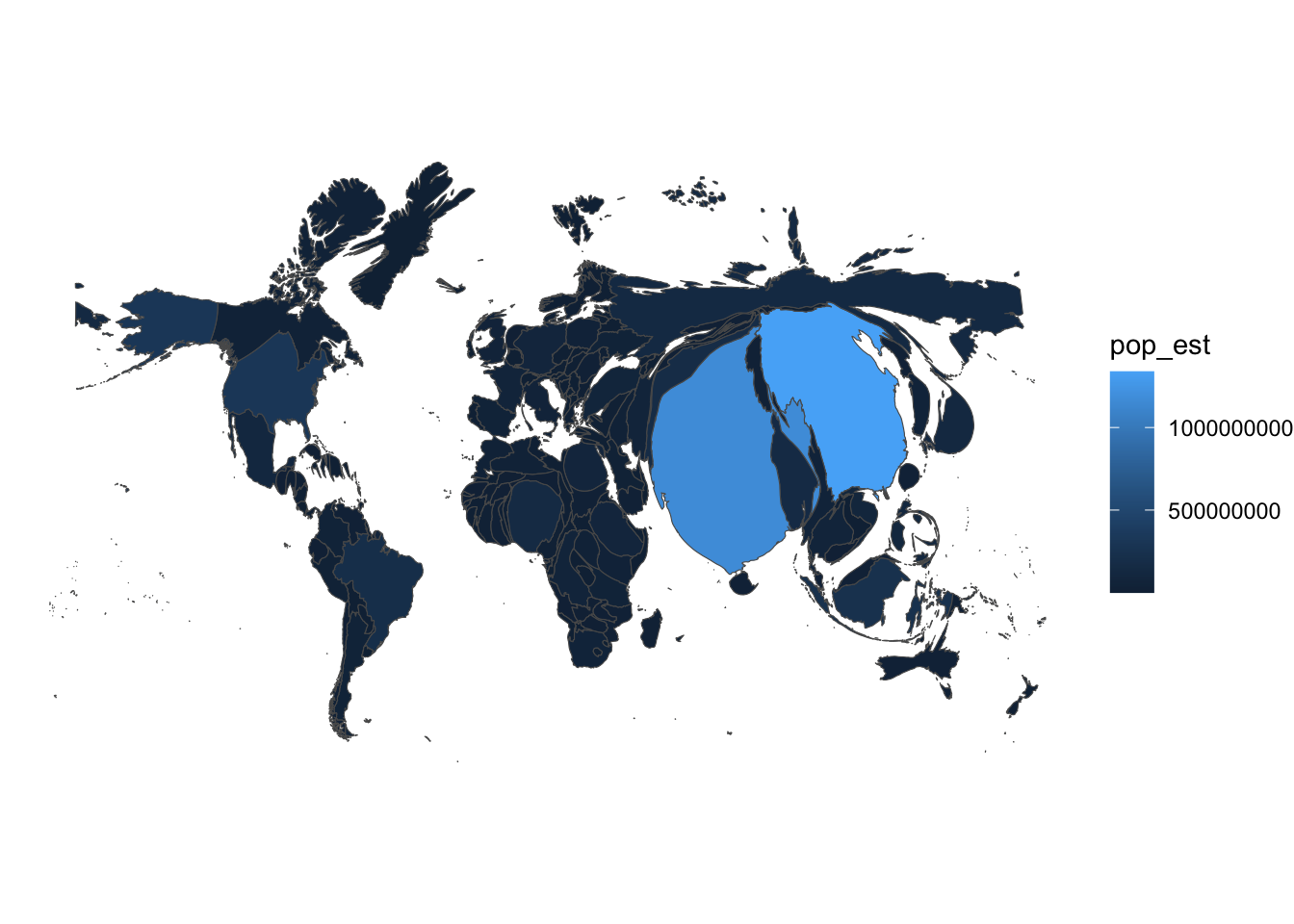
viridis) Colorsggplot(mapdata_cartogram) +
geom_sf(aes(fill = pop_est)) + # fill is population estimate
scale_fill_viridis_c(name = "population",
option = "viridis") + # beautiful colors
theme_void()