Show the code
library(readr) # read CSV

library(dplyr) # data wrangling

library(sf) # simple features
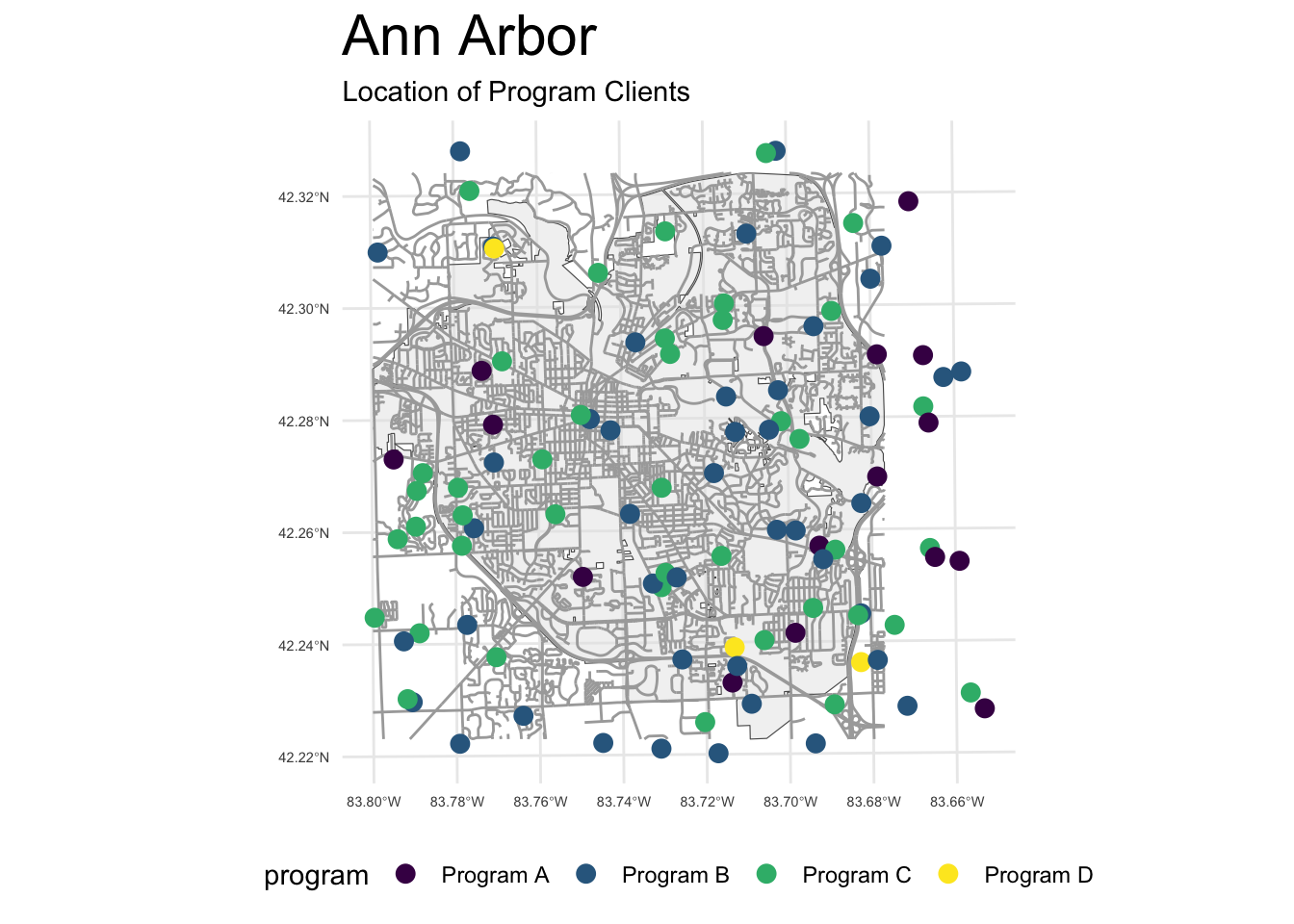
library(ggplot2) # mapsggplot Using Location DataSometimes we have map data that come in the form of location data where the latitude and longitude (Chapter 4) of each participant or location is listed in the data set.
Below I describe the process of working with such location data. Location data can easily be combined with shapefiles (Chapter 8) in ggplot.
library(readr) # read CSV
library(dplyr) # data wrangling
library(sf) # simple features
library(ggplot2) # mapsread_csv to Read Text File with Client Dataclients <- read_csv("./location-data/clients.csv")clients <- clients %>%
filter(latitude <= 42.33 &
latitude >= 42.22 &
longitude >= -83.8 &
longitude <= -83.65)sf Object While Indicating Coordinate Reference System (CRS)point <- st_as_sf(clients,
coords = c("longitude", "latitude"),
crs = 4269) # A2 is NAD1983
# write to shapefile
st_write(point,
"./shapefiles/clients/clients.shp",
append = FALSE) # replace; don't appendcity_boundary <- read_sf("./shapefiles/AA_City_Boundary/AA_City_Boundary.shp")
WashtenawRoads <- read_sf("./shapefiles/Roads/RoadCenterlines.shp")
AnnArborRoads <- st_crop(WashtenawRoads,
city_boundary) # crop to only get A2 roadsggplot(city_boundary) +
geom_sf(alpha = .5) +
geom_sf(data = AnnArborRoads,
color = "darkgrey") +
geom_sf(data = point,
aes(color = program),
size = 3) +
labs(title = "Ann Arbor",
subtitle = "Location of Program Clients") +
scale_color_viridis_d() +
scale_fill_viridis_d() +
theme_minimal() +
theme(plot.title = element_text(size = rel(2)),
axis.text = element_text(size = rel(.5)),
legend.position = "bottom")