5  Map Projections

5.1 Introduction

Map projections exist because we are trying to take the round globe of the earth, and project it onto a 2 dimensional surface. Because a spherical globe can not be projected onto a flat surface without some distortion, different projections make different choices about the kind of distortion involved.

A Flat Map

A Globe

5.2 Call The Libraries

library(rnaturalearth) # natural earth data

library(ggplot2) # beautiful maps

library(dplyr) # data wrangling

library(sf) # simple (spatial) features

5.3 Get The Data

mapdata <- ne_countries(scale = "medium", # medium scale
                        returnclass = "sf") # as sf object

5.4 A Basic Map

mymap <- ggplot(mapdata) + # the data I am mapping
  geom_sf() + # the geometry I am using
  theme_minimal() + # minimal theme
  theme(axis.text.x = element_blank()) # no longitude labels

mymap # replay

5.5 Map Projections

5.5.1 Globe (Orthographic)

Key Idea

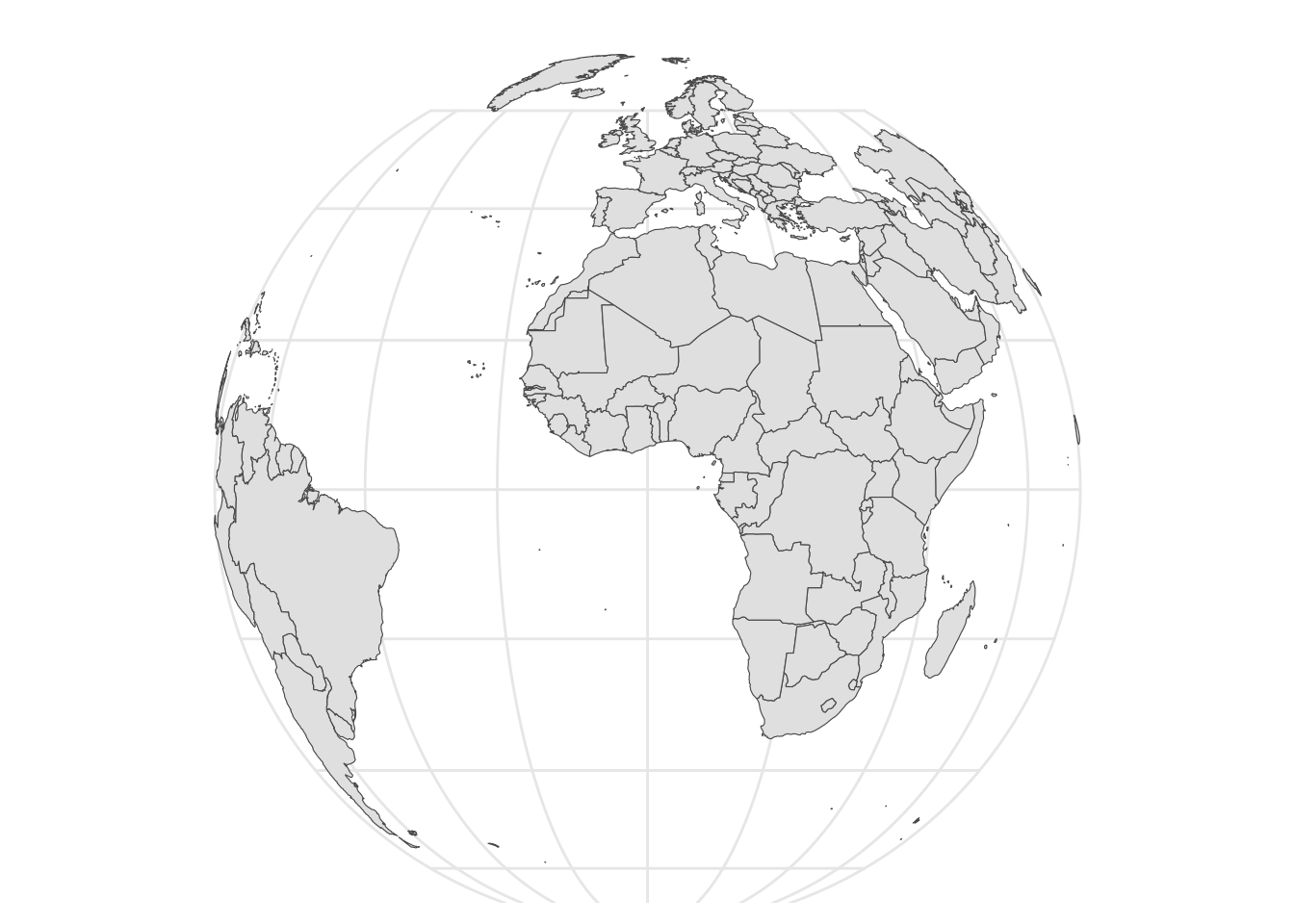
An orthographic projection represents the globe as a 3 dimensional view.

mymap + coord_sf(crs="+proj=ortho")

5.5.2 Mercator

Key Idea

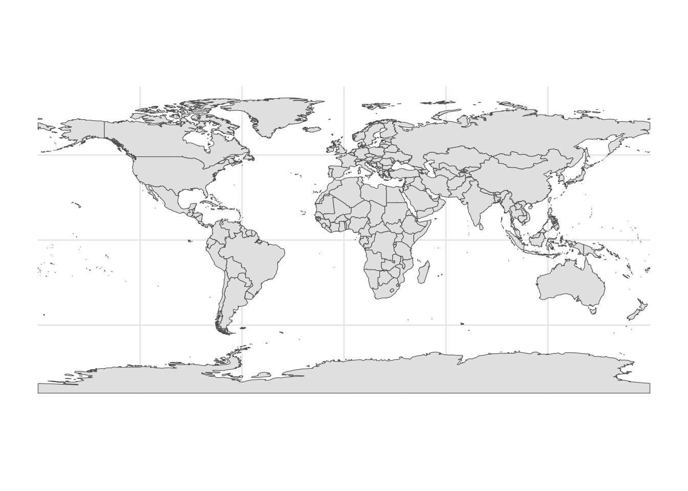
A Mercator projection represents the earth with perpendicular latitude and longitude. This projection can be helpful in some kinds of navigation, but areas of landmasses are distorted. As one approaches the poles, landmasses are over-sized, while landmasses closer to the equator are under-emphasized. Thus, this projection is often seen as one that does not properly acknowledge the size of countries in the Global South.

Antarctica can often not be correctly mapped with the Mercator projection. One way to avoid this difficulty is to employ a slightly more complicated procedure, removing Antarctica from the data before plotting.

mercator_data <- mapdata %>% 
  filter(name != "Antarctica") # remove Antarctica

ggplot(mercator_data) + # the data I am mapping
  geom_sf() + # the geometry I am using
  coord_sf(crs = 3857) + # Mercator
  theme_minimal() + # minimal theme
  theme(axis.text.x = element_blank()) # no longitude labels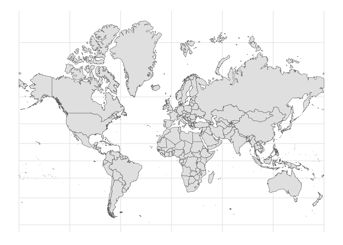

5.5.3 Mollweide

Key Idea

The Mollweide projection is an equal area projection. As a consequence, latitude and longitude lines are not perpendicular, and the shapes of some landmasses may appear to be distorted.

mymap + coord_sf(crs="+proj=moll")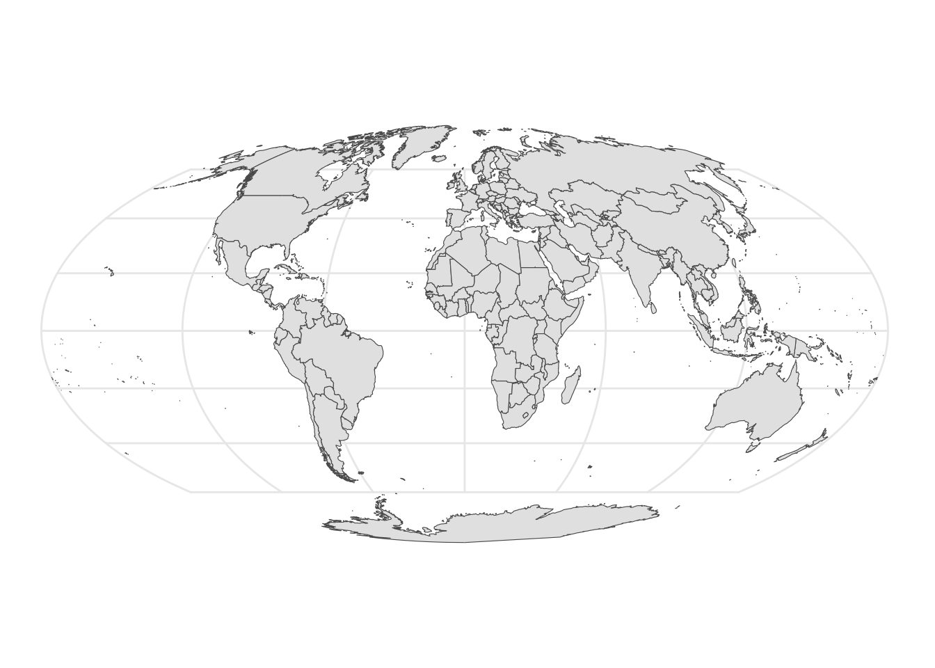

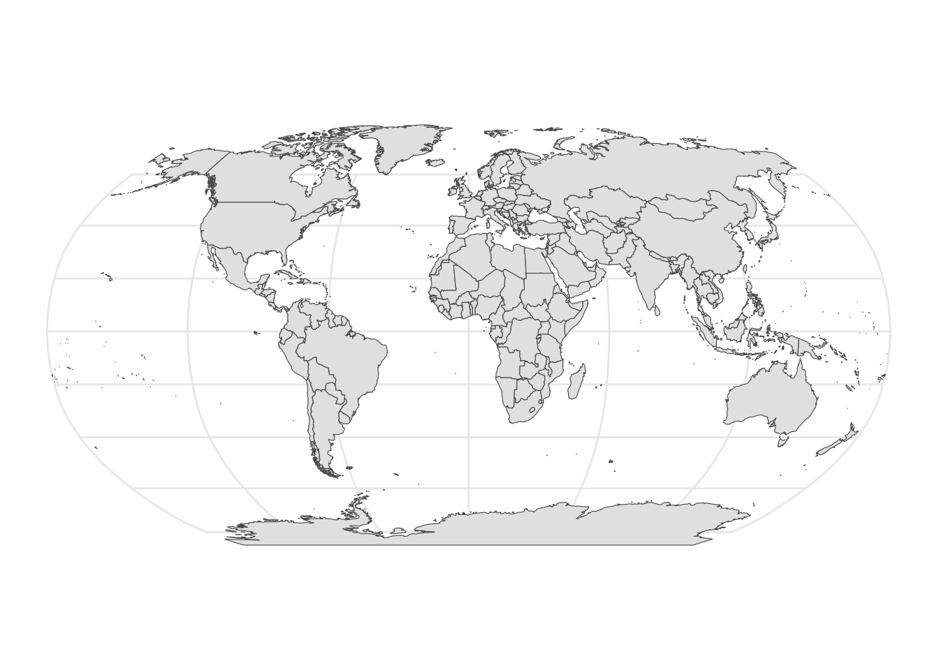
5.5.4 Robinson

Key Idea

The Robinson projection is an attempt to compromise between equal areas and a natural looking map.

mymap + coord_sf(crs="+proj=robin")