12 Making Maps with `ggplot`

12.1 Call the libraries

Code

library(ggplot2) # beautiful graphs

library(dplyr) # data wrangling

library(sf) # simple (spatial) features

library(readr) # import csv

12.2 Use `read_sf` To Open Shapefiles

Getting the directory and filename right is important.

Code

city_boundary <- read_sf("./shapefiles/AA_City_Boundary/AA_City_Boundary.shp")

buildings <- read_sf("./shapefiles/AA_Building_Footprints/AA_Building_Footprints.shp")

trees <- read_sf("./shapefiles/a2trees/AA_Trees.shp")

parks <- read_sf("./shapefiles/AA_Parks/AA_Parks.shp")

university <- read_sf("./shapefiles/AA_University/AA_University.shp")

WashtenawRoads <- read_sf("./shapefiles/Roads/RoadCenterlines.shp")

AnnArborRoads <- st_crop(WashtenawRoads, 
                         city_boundary) # crop to only get A2 roads

Warning: attribute variables are assumed to be spatially constant throughout
all geometries

Code

# watersheds <- read_sf("../shapefiles/watersheds/Watersheds.shp")

12.3 Use `ggplot` to Make The Map

Code

# NB RE Macs: the plotting device on Macs can be very slow
# we notice this with all the detail that is involved in maps
# maps can be REALLY slow on Macs
# so--inconveniently--we write directly to PDF on a Mac
# and don't see the graph in our RStudio window
# we have to manually open the PDF to see the created map

# Apparently, the first layer is important for setting the CRS of the map

# pdf("./mapping/ggplot-map-test.pdf") # open PDF device (uncomment on Mac)

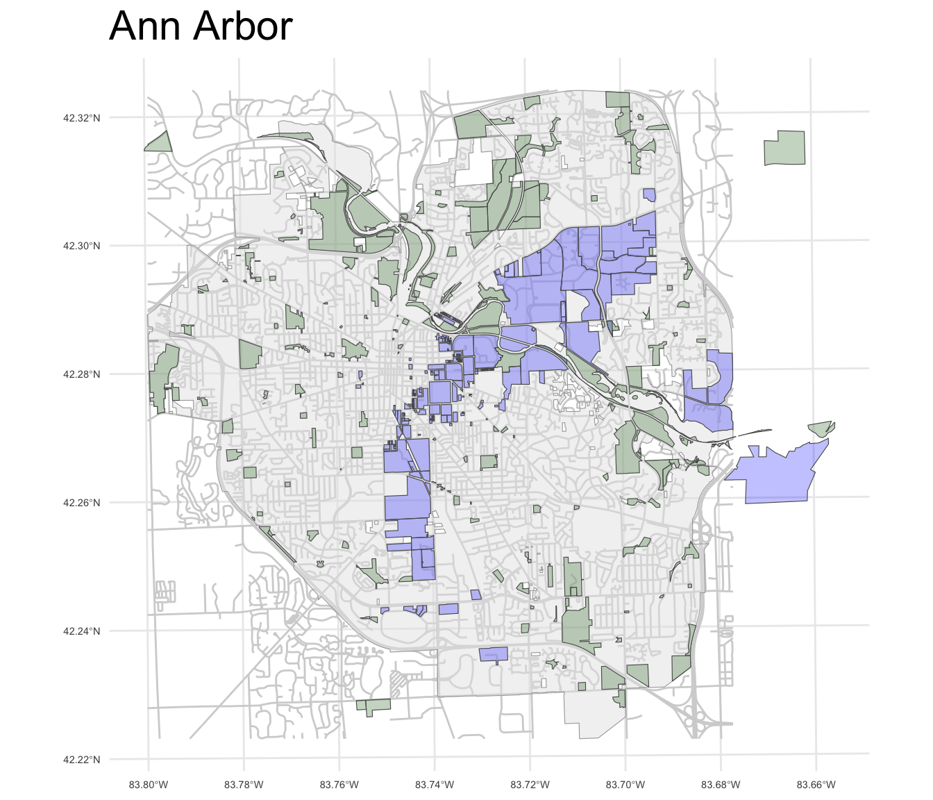
# dev.off() # turn off PDF device (uncomment on Mac)

Code

ggplot(city_boundary) +
  # geom_sf(data = buildings,
  #         fill = "lightgrey") +
  geom_sf(data = AnnArborRoads, 
          color = "lightgrey") +
  geom_sf(color = "darkgrey", alpha = .5) +
  geom_sf(data = university, 
          fill = "blue", 
          alpha = .25) + 
  geom_sf(data = parks, 
          fill = "darkgreen", 
          alpha = .25) +
  # geom_sf(data = trees, 
  #         size = .1,
  #         color = "darkgreen") +
  labs(title = "Ann Arbor") +
  scale_color_viridis_d() +
  scale_fill_viridis_d() +
  theme_minimal() +
  theme(plot.title = element_text(size = rel(2)), 
        axis.text = element_text(size = rel(.5)),
        legend.position = "bottom")